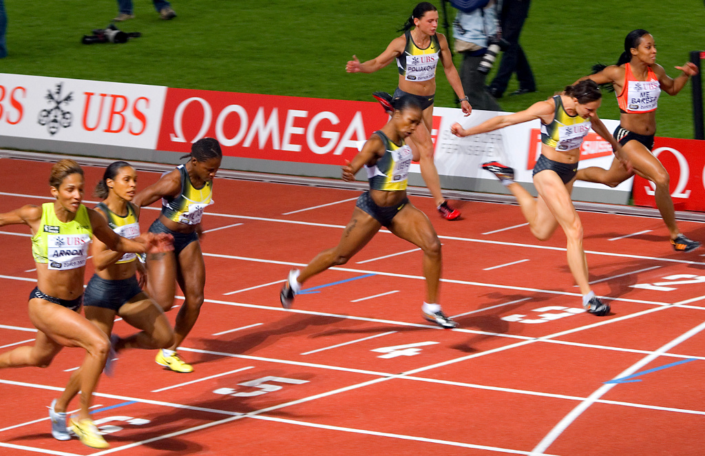
Kinematics is
the study of motion without considering its causes. In the
case of the runners in the photograph, the motion of their
legs and arms is oscillatory, while their heads' motion is
more similar to rectilinear uniform motion being then easier
to describe; it would be enough to follow the horizontal
displacement of a point in the head at different
instants. To describe the motion of the legs, besides the
horizontal displacement, it would also be necessary to
measure an angle at different instants.
1.1. Rigid bodies motion
An object is in motion if its position is different at different
instants; if the position remained the same, the object
would be at rest. To
determine the position of an object it is necessary to use
a reference
frame; namely, other objects used as reference. If
the position of the object changes with respect to that
reference frame, the body has motion relative to that
frame. Therefore, motion is a relative property, since a
body can be in motion relative to a reference frame and also
at rest relative to another reference frame.
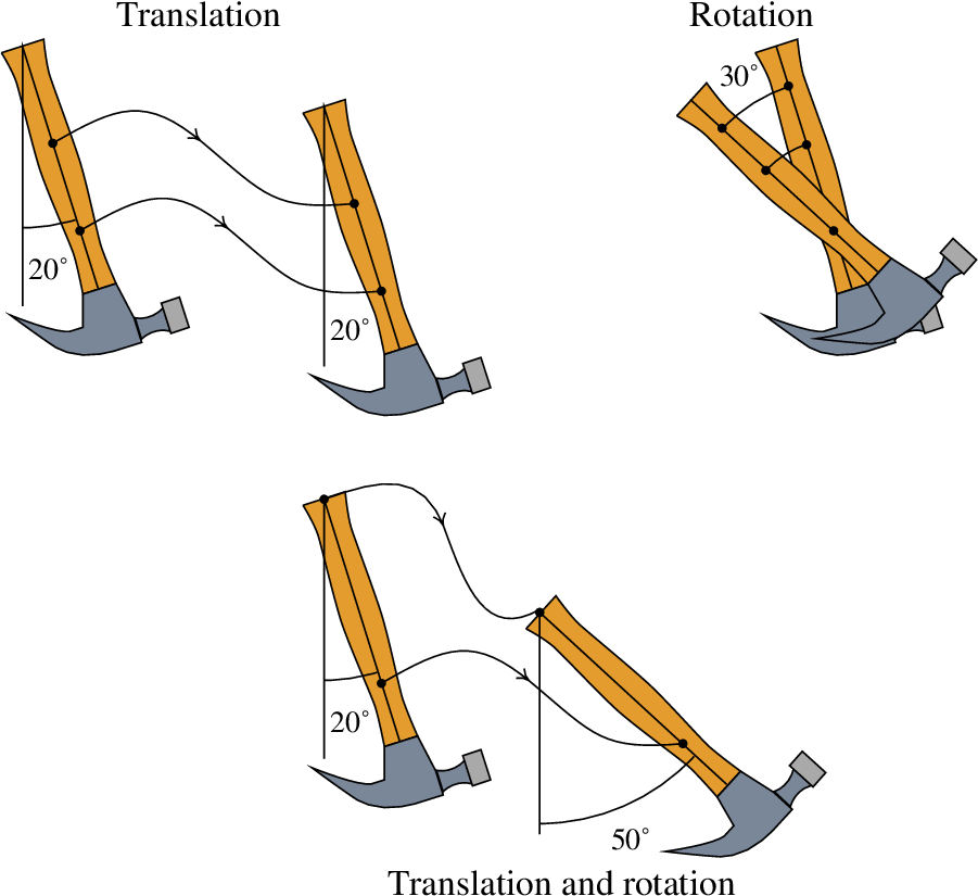
The simplest motion that a rigid body can have is a
translation without rotation, when all of its parts follow
exactly the same trajectory (see
Figure 1.1). Hence, in that case
it would suffice to describe the motion of a single point in
the body in order to follow the motion of the
whole rigid
body.
Figure 1.1: Translation, rotation around a fixed
axis and the combination of those two
motions.
In the rotation around a fixed axis, all the points in an
axis remain at rest and the other points move. In the second
part of Figure 1.1, the hammer
rotated around an axis perpendicular to the page. The
trajectories of different points are no longer the same, but
they are all circular arcs, with the same angle, which only
differ in the length of the radius. It would be enough to
know how the angle changes with time, in order to describe
the motion of any point in the body.
A more complicated motion is obtained from the
superposition of a translation and a rotation around a fixed
axis (third part in
Figure 1.1). In that case, the
trajectories of different points are all different
curves. However, that complicated motion can be obtained
from the trajectory of any point in the body and the
rotation of any line segment in the body (not parallel to
the rotation axis). All line segments in the body rotate at
the same rate and once the position of the reference point
and the rotation angle are known at a given instant, the
position of all other points in the body can be found at
that instant.
There is also a more general type of rotation, around a
point, in which the direction of the rotation axis changes
with time. In that case the trajectories of all points
relative to a reference point will be different curves on
the surfaces of spheres centered in that point. A convenient
way to describe that kind of motion consists in using two
angles to determine the direction of the axis; together with
the rotation angle around that axis, a total or three angles
are needed in addition to three distances to determine the
position of the reference point.
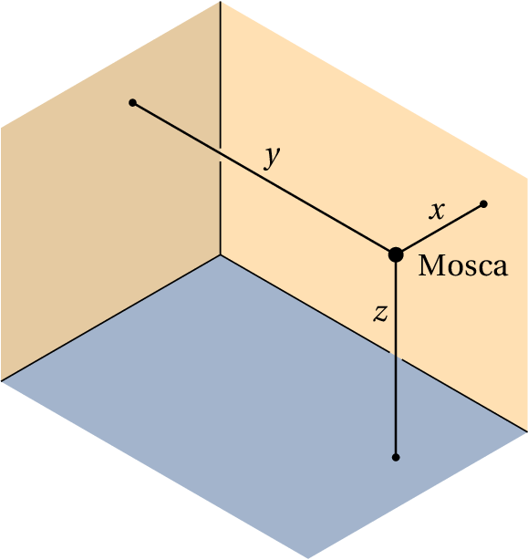
1.2. Motion and degrees of freedom
The degrees of freedom of a system are
the variables needed to determine its exact position. For
example, to determine the position of a fly in a
"rectangular" room, its distance to the floor and
to two perpendicular walls can be measured, giving rise to a
system of perpendicular coordinates (Cartesian or
rectangular coordinates), which are usually labeled with the
three letters
,
and
(figure 1.2).
Figure 1.2: Cartesian coordinates of a fly in a
rectangular room.
That means that the motion of a point in space has 3
degrees of freedom. The trajectory of the point is a curve
in space, which can be described by 3 expressions for the 3
Cartesian coordinates
,
and
as functions of
time. Since the most general motion of a rigid body can be
described by the change of three angles and the motion of a
point, that kind of motion has 6 degrees of freedom. Other
simpler motions of a rigid body have less degrees of
freedom; the rotation around a fixed axis has only one
degree of freedom, translation without rotation has 3
degrees of freedom and the superposition of translation and
fixed axis rotation has 4 degrees of freedom.
The subject of study in this chapter is the motion of a
single point, which will be enough in order to study the
translation of rigid bodies and will be the basis to study
their general motion.
When a point is restricted to move along a predetermined
curve, the motion of that point has only one degree of
freedom. For instance, the motion of each wheel of a cart in
a roller coaster will follow the curve of the tracks, as
long as the cart does not fall off the tracks, so the center
of the wheels will follow a known curve. Given the position
of that point at an initial instant, to find out the
position at a later instant it will be enough to know the
distance that the point moved along its trajectory.
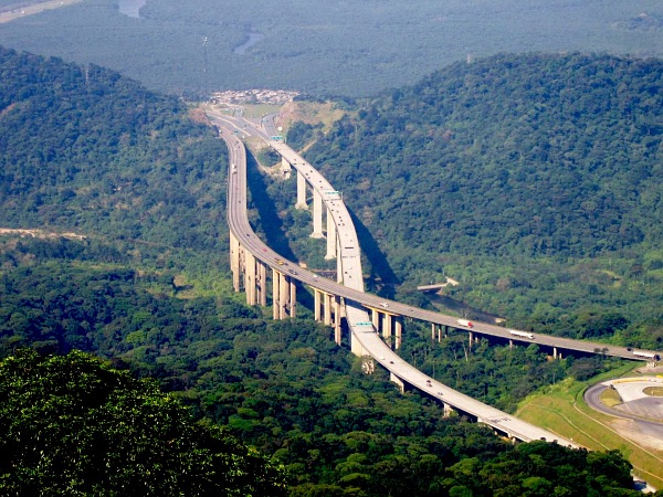
When a car moves on a road, one single degree of freedom
might be enough to describe its motion
(Figure 1.3). If the car breaks
down and the driver has to call a towing truck, it will be
enough to tell the truck driver the road where the car is
and the kilometer along that road. Hence, the motion of cars
on a road has one degree of freedom, which is the
displacement along the road.
Figure 1.3: The translation of a car along a road
can be described with only one degree of freedom.
It must be pointed out that the displacement along the road
is not measured in a straight line, but along a curve in
space; however, since that curve is fixed, only one variable
is enough to establish the position at a given instant. In
some cases it might become necessary to describe the
variation of other degrees of freedom, for instance, the
distance from the car to the road's edge. If the car was
perfectly rigid and its wheels remained always in contact
with the road's surface, the complete description of it s
motion would also require an angle. In practice, there are
always many degrees of freedom because objects are never
perfectly rigid.
If a point is constrained to move on a surface, two
coordinates will be enough to determine its position and
thus, its motion has two degrees of freedom. A biologist
tacking the motion of a fox in a region will only need to
measure its latitude and longitude, for instance with a GPS
device, in order to know where it is at different
instants. Only 2, rather than 3, coordinates are needed
because the topography of the terrain is known, as in
Figure 1.4, making it possible
to determine its exact position just from its latitude and
longitude; there is really a third coordinate, the height
over the terrain, but since its variation might be
insignificant when compared with the variations in the
latitude and longitude, it will probably be irrelevant to
the study.
Figure 1.4: The translation on the surface of a
terrain is a motion with two degrees of freedom.
Therefore, the translation of the fox has two degrees of
freedom, because two variables are enough to determine its
position. The latitude and longitude are not really
distances but angles with their vertices at the center of
the Earth, but they are degrees of freedom because can have
different values at different instants.
Going back to the example of the fly in a room, which was
regarded as having only three degrees of freedom
,
e
, the fly can also change its orientation in space. To
determine its orientation in any instant 2 angles might be
used and a third angle is needed to determine its rotation
along that axis. And since the fly can also stretch or bend
its body and open or close its wings, from a mechanical
point of view it has several degrees of freedom. If it was
modeled by three rigid bodies: two wings and the block
formed by its abdomen, thorax and head, 6 degrees of freedom
would be needed to describe the motion of that block; each
wing will add other 3 degrees of freedom — the three
rotation angles with respect to the point where the wing
joins the thorax — leading to a total of 12 degrees of
freedom.
1.3. Displacement and velocity
This chapter deals only with motions with a single degree
of freedom, when the trajectory is a known curve. To
determine the position along the trajectory, a variable
is used, which is measured from a point chosen as the origin
(where
); the points on one side of that
origin are given positive values of
and the points on
the other side are given negative values of
.
The position
is a function of time, because at each
instant the point can be in one position only and it is a
continuous function because the point cannot move from one
position to another without first passing through all the
positions in between. At an instant
later than
(
), the point will be in another
position
. The increment of its position
during that time interval
is
called displacement and it is given by
(1.1)
The average
velocity, during that time interval is defined as
the displacement divided by the time interval
(1.2)
The displacement and the average velocity can be positive
or negative, but both have the same sign. If they are
positive, it means that the motion is in the positive
direction (in which
increases) and if they are negative,
the motion is in the negative direction. The absolute value
of
is the average
speed of the
object. Velocity and speed are measured in units of distance
over time; for instance, meters per second, m/s, or
kilometers per hour, km/h.
Example 1.1
A car driver registered his position in a highway at
several instants, obtaining the data shown in the
table.
time (h)
0
0.5
1.0
1.5
2.0
distance (km)
0
60
90
100
140
Compute the average velocity in each half-hour interval
and make the plots of position vs time and average
velocity vs time.
Solution. If
,
, ...,
are the five
instants registered in the table, the average velocities in
the four intervals are the following
The plot of position vs time can be made
with Maxima
(see appendix A). It
is convenient to save the time and position data into a list
that will then be used to make the plot with function
plot2d.
The result is shown in
Figure 1.5. Since
should
be a continuous function, its plot should be a curve that
goes through the points shown in the figure; however, the
information given is not enough to know that curve.
Figure 1.5: Plot of position on the trajectory at some
instants.
To plot the average velocity with respect to time, it
should be kept in mind that each average velocity was
computed for a time interval and, hence, each value obtained
should be associated to all the instants in that
interval. The following two commands create a list with the
average velocities with respect to time that is then used to
make the plot using plot2d. It is
not necessary to use option style,
because by default the points given will be connected by
line segments.
Figure 1.6: Plot of the average velocity in
several time intervals.
The plot 1.6 does not provide
precise information about the true motion of the car. For
instance, in the second time interval from 0.5 to 1 hour,
instead of traveling at a constant velocity of 60 km/h,
as the plot suggests, the driver might have kept the
120 km/h velocity of the first half hour during 15
minutes and then stop for the remaining 15 minutes in that
interval; thus, during the first 15 minutes of that second
interval the car would have traveled 30 km, reaching
the
km position registered in the
table.
The position is calculated from the average velocity by
combining equations 1.1
and 1.2
(1.3)
The second term in this last equation is the displacement
during the time interval
. Splitting that interval into
subintervals, this last equation would become
(1.4)
Where
is the average velocity in the
subinterval. Therefore, the average
velocity of 60 km/h in the interval
h, leads to a
displacement
km,
which is the same that would be obtained with an average
velocity
km/h during
h, followed by a
second average velocity
, during
h.
But the velocity cannot change instantly from 120 km/h
to 0 without passing through all the values between 120 and
0. In other words, velocity is also a continuous function of
time,
, as it is the case for position
. To get
a better glimpse of the two functions
and
, the
time interval
can be divided in many more
subintervals and the position should be measured in all
those subintervals. In the limit when
goes to infinity,
the sum in equation 1.4 is called
an integral and
the following notation is used
(1.5)
Within the integral,
without a bar over it stands for the
instantaneous velocity
,
equal to the limit of the average velocity as the time
interval approaches zero
(1.6)
This limit is called derivative; the last part of the
equation shows a notation used very often for the
derivative. In this case it is the derivative of function
(position) with respect to
(time). In this book
another notation will be used more often, in which a
derivative with respect to time is indicated by writing a
dot on top of the function
(1.7)
Hereafter for the sake of simplicity, the instantaneous
velocity at an instant
will always be called simply
velocity.
In a car, the instantaneous speed (absolute value of the
instantaneous velocity) is measured with a good
approximation by the speedometer. The speedometer reading
will have some error associated with the minimum response
time of the device,
. A good quality
speedometer should have a very small response time; also,
the slower the speed changes, the more accurate the reading
of the speedometer will be.
1.4. Acceleration
Following the same argument that led to the definition of
instantaneous velocity, the increment of
during a time
interval
is given by
(1.8)
And the
average
tangential acceleration is the velocity
increment divided by the time interval
(1.9)
These last two equations can be combined to give the
velocity at a later instant, in terms of the initial
velocity and the average tangential acceleration
(1.10)
Dividing the time interval into subintervals that approach
zero, the velocity is then found by integrating the
instantaneous tangential acceleration
(1.11)
Where the instantaneous
tangential acceleration equals
the derivative of the velocity with respect to time and,
therefore, it is also equal to the second derivative of
the position with respect to time
(1.12)
The acceleration has units of distance over time
squared. For instance, meters per second squared,
m/s2.
A negative tangential acceleration means that the velocity
is decreasing: it might be slowing down, if the motion is in
the positive direction, or it might be speeding up if the
motion is in the negative direction. Positive tangential
acceleration implies that the point is speeding up, if its
motion is in the positive direction, or slowing down if it
moves in the negative direction. Zero tangential
acceleration implies uniform motion (constant velocity)
The term "tangential acceleration", instead of
just acceleration, is being used because as it will be
explained in
chapter 3, this
is only one component of the acceleration which also has
another component perpendicular to the trajectory. On the
other hand, the velocity always follows the direction of the
trajectory and for that reason there is no need to call it
tangential velocity.
The tangential acceleration is also a function of time, as
well as position and velocity. However, unlike position and
velocity, the tangential acceleration does not have to be a
continuous function. Position and velocity are properties
that define the state of an object and that state cannot
suffer abrupt changes, while the acceleration is related to
external factors that can suddenly appear or
disappear. Hence, the derivative of the acceleration will
not be defined as another physical quantity.
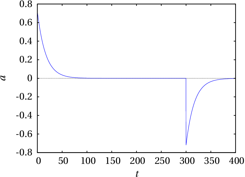
Example 1.2
A ship is initially at rest in a channel; at an instant
= 0 the engine is turned on during 5 minutes and it is
then turned off, letting the ship come to a stop due to
the water resistance. The expression for the velocity as a
function of time
, in SI units, is
Find the expressions for the tangential acceleration and
the position in the trajectory as a function of time. Plot
the velocity, tangential acceleration and position with
respect to time. Compute the distances traveled by the
ship while the engine was on and after it was turned
off.
Solution. First, notice that the expression given
for the velocity is a continuous function as it should
be. The tangential acceleration is obtained differentiating
the expression for the velocity. In order to make the
computation in Maxima, one can start by saving the two
expressions given for the velocity into two different
variables
Notice that the tangential acceleration is discontinuous in
this case. At
, the
expression a1 approaches
,
which is a positive number, while a2 approaches
, which is negative. There is
a discontinuity in the acceleration at
s,
because at that instant the engine was suddenly turned
off.
To obtain the expression for the position at any instant
, equation 1.5 is used,
replacing the initial instant
by 0 and the final instant
+
by
; the initial position
can be chosen as equal to 0. For
less than or equal to
300, the expression that should be integrated is the first
expression given for
For
greater than 300 the initial time in
equation 1.5 can be fixed as 300
and the initial position becomes
, given by the
expression for
, and the second expression given for
should be integrated
Those two integrals are computed in Maxima as follows
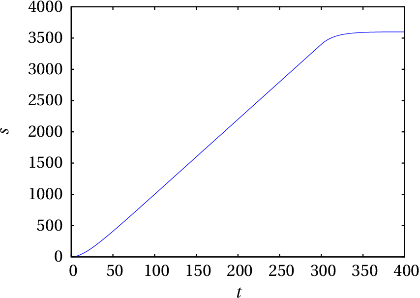
Figure 1.9: Plot of the position in the
trajectory.
The plots provide useful information that is less obvious
in the algebraic expressions. The plot of the velocity shows
that the ship quickly approaches a maximum velocity of
around 12 m/s during the first minute, which remains
constant until the moment when the engine is turned
off. From that moment on, the velocity decreases quickly and
at
s (6 minutes) it is practically zero.
The plot of the tangential acceleration shows that when the
motor is turned on, it produces an acceleration of
approximately 0.7 m/s2 that quickly
decreases. When the motor is switched off, the tangential
acceleration suddenly becomes approximately
−0.7 m/s2 and the way its absolute value
decreases with time appears to be identical to the way the
initial positive acceleration decreased, the reason being
that both acceleration decreases are due to the water
resistance. That similarity of the plot of the acceleration
when the motor is turned on and when it is turned off,
implies that the area between the curve for
and the
axis is the same in both cases; therefore, the
integral of
while the motor was on and off
are both equal, but with opposite signs and that implies
that the speed that the ship gains while the motor is on
equals the speed that it looses until it stops, as it should
be.
In practice, the expression given for the velocity cannot
be completely true when it leads to small values; for
instance, at
s the expression for the
velocity gives
(%i14) float (subst (t=400, v2));
(%o14) 0.02975
almost 3 centimeters per second. There are other factors,
such as water currents, wind and waves, that will introduce
velocity variations greater than that value. The expression
given is a mathematical model that is only valid when all
those other factors can be neglected.
The discontinuity on the plot of the tangential
acceleration at
s appears as a vertical
segment because Maxima's command
plot2d does
not discover the discontinuity at that point, but regards
the two parts in the plot as a single continuous
function. The plot of the position shows a linear
increase in almost all of the first 5 minutes. The
distance traveled while the motor was turned on equals
the displacement from
to
; since the
initial position is
, that displacement is
According to the theoretical model, the ship would take an
infinite time to stop; in practice, it stops after about 6
minutes, as it was discussed above. As such, the distance
traveled after the motor was turned off would be
. The limit of
as
approaches
infinity is calculated in Maxima as follows
(%i15) limit (s2, t, inf);
(%o15) 3600
It is then concluded that the ship travels 200 m since
the engine is turned off until stops.
1.5. Uniform and uniformly accelerated motion
A motion is called uniform if the velocity remains
constant. Since the derivative of a constant is zero, the
tangential acceleration is then zero. The result obtained
from equation 1.4 will be the
same, independently of the number of subintervals, because
is the same in all the subintervals (the average
velocity equals the velocity in this case) and that result
is
(1.13)
where
is the position at instant
,
is the
initial position at
e
the velocity,
which is the same at any time.
A uniformly accelerated motion is one which
has a constant tangential acceleration. In that case, the
average tangential acceleration in
equation 1.10 can be replaced by
the constant value of the tangential acceleration leading
to
(1.14)
where
is the velocity in
. The
expression for the position is obtained by substituting this
equation into equation 1.5
(1.15)
The time
can be eliminated from
equations 1.14 and
1.15, leading to an expression that relates
velocity and position
(1.16)
It should be remembered that
equations 1.14,
1.15 and 1.16
are only valid in the case of a constant tangential
acceleration. When the tangential acceleration is not
constant, in order to obtain an expression for the velocity
from equation 1.11 it would be
necessary to know
as a function of
. And
the expression obtained for
could then be integrated in
equation 1.5, leading to an
expression for
which will not have the same quadratic
form 1.15. If the expression for
as a function of time is not known, in some
cases the method explained in the next section can be
used.
1.6. Kinematic equations
The differential equations1.7 and 1.12
define the relation among the kinematic variables (
,
,
) and the time
. If the expression for one
of those variables as a function of time is known, the
expressions for the other two variables can be found just by
differentiation or integration, as it was done in the
example 1.2.
When an expression for
as a function of
is known,
the derivative of
with respect to
can be obtained
by the rule for differentiation of composed functions
(1.17)
This is another relation among three of the four kinematic
variables. To summarize, the four equations that relate
three of the four kinematic variables
,
,
and
are (notice that the equations with dots
include the variable
)
(1.18)
Any of those equations can be solved when there is a known
relation among some of the three variables in the
equation. For instance, let us consider the first equation,
; if an expression for the position in terms of
time is known, namely
, the equation becomes
(1.19)
which implies that the expression for
in terms of
is the derivative
of the function given. Notice
that if the function
depended on other variables, for
instance
or
, the velocity
would not
be just the derivative of
, since the derivative must be
computed using the the chain rule:
(1.20)
In the first case, an expression for the acceleration in
terms of the velocity is obtained and in the second case one
only finds a relation involving the acceleration, the
velocity and the time. In cases when an expression for
in terms of
is known,
, as in the
example 1.2, the equation becomes
In more complicated cases, for instance if the relation
known is of the form
, it is obtained an
ordinary differential equation, namely, an
equation with two variables and the derivative of one of
them with respect to the other. A similar analysis can be
made with the other 3 equations.
Some differential equations can be solved analytically
using various known methods, as shown in the next example,
but in some other cases the solution must be obtained
numerically, which will be discussed in chapter 7.
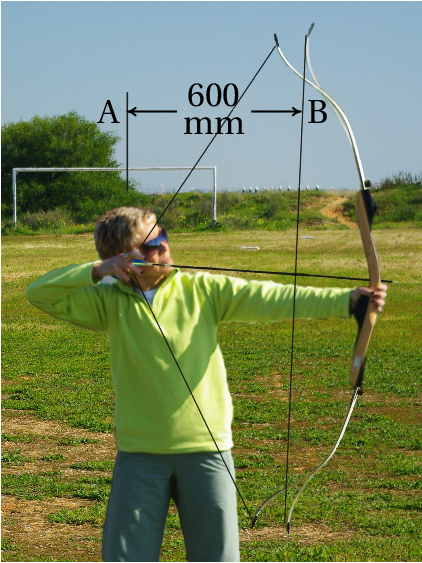
Example 1.3
When an arrow is thrown with a bow (see the figure),
while the arrow is in contact with the string its
tangential acceleration decreases linearly with respect to
its position
, from a maximum value of
4500 m/s2, when the back of the arrow is
in the initial position A, down to zero when it reaches
the point B where the bow recovers its normal shape. The
distance between points A and B is 600 mm. Determine
the velocity of the arrow as it leaves the bow in B.
Solution: Using point A as the origin for the
position
of the arrow and SI units, the expression for
the tangential acceleration in the interval 0 ≤
≤
0.6 m is the equation of the straight line that goes
through points (
,
) = (0, 4500) and (
,
) = (0.6, 0), namely
This expression can be substituted in the equation
leading to an ordinary differential equation
Moreover, this kind of equation is
called separable, because the two
variables can be separated in the two sides of the equation
in the following way
If
= 0 is chosen as the instant when the arrow is
released at point A, then the initial condition necessary to
solve this equation is that
= 0 when
=
0. Integrating on each side of the equation, from those
initial values up to the values in point B, one has
Notice that the limits in both integrals must be
consistent; namely, each limit in the integral with respect
to
is the value of
in a point and the corresponding
limit in the integral with respect to
on the other side
of the equation is the value of
at that same point.
Solving the two integrals, the value of
at point B is
obtained
1.6.1. Projection along a straight axis
In some cases it is more convenient to study the motion
of a point along a curve by studying the motion of its
projection along a straight line which is considered, for
instance, the
axis.
In an interval
, the displacement of
the projection along the axis will be
. Therefore, the derivative
of
the
projection with respect to time is the projection
of the velocity along the axis,
. And the derivative
is the projection of the acceleration along
the axis,
. Notice that
= 0 does not imply
zero velocity, because it might happen that the trajectory
is perpendicular to the axis at some point, making the
projection of the velocity equal to zero in that point.
Also,
is the projection of the total acceleration
and not only its tangential component; for instance,
can be constant, implying
equal to zero,
but if the trajectory is curved, the
projection of
can be different at different points, implying that
is not equal to zero.
The equations that relate
,
,
and
are
similar to the equations 1.18
for the motion along the trajectory
(1.23)
In the particular case of rectilinear motion, when the
trajectory is a straight line, and if the
axis is
chosen parallel to the trajectory, then
is equal to
the position
in the trajectory,
is the velocity
and
is the total acceleration, rather than just
its tangential part. The axis can be called
,
or
anything else instead of
.
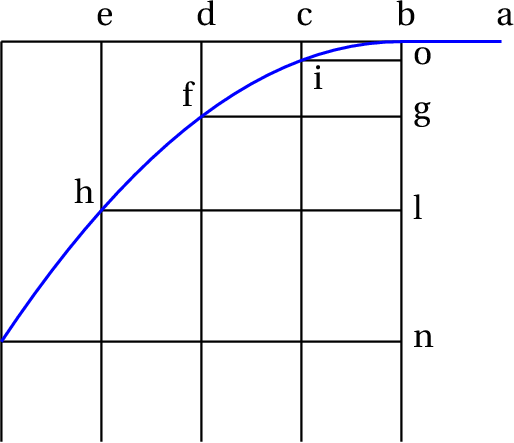
1.6.2. Acceleration of gravity
As Galileo Galilei explained in his book of 1638,
"Dialogues Concerning Two New Sciences", the
motion of a projectile thrown in the air can be
conveniently decomposed into two motions: the motion of
the its projection along the horizontal plane, and the
motion of its projection along a vertical
axis. Figure 1.10 is the same original figure 108
from Galileo's book of an object that was thrown from
point a on a horizontal surface, leaving that surface at
point b.
Figure 1.10: Trajectory of a projectile, as explained by
Galileo.
Galileo also discovered that when the air resistance can
be neglected, which is true when the object has a compact
shape and its trajectory in the air is not too long, the
motion of the horizontal projection is rectilinear and
uniform, namely, in equal intervals of time the object
moves from a to b, then from b to c, from c to d and from
d to e. In the vertical direction, the distance the
projectile falls in equal intervals of time increases
quadratically; namely, during the first interval it falls
the distance
, during the second interval
it has already fallen the distance
, which
is four times bigger than
and during the
third interval the distance
, which is nine
times bigger than
. Thus, the vertical
projection of the acceleration is constant.
When the air resistance can be neglected, all objects,
independently of their size and masses, are accelerated
downwards with the same acceleration , called gravity. The vertical
projection of the motion is a uniformly accelerated
motion, while the horizontal projection is a uniform
motion.
The value of the acceleration of gravity is slightly
different in different places on Earth, but it is
approximately 9.8 m/s2.
If the vertical is represented by the
axis, pointing
upward, then the vertical projection of the acceleration
is
m/s2 and its
horizontal projection is
= 0.
Example 1.4
A stone is thrown from a bridge that is 5 m above
the surface of a river, with an initial velocity of
15 m/s at an angle of 36.9° over the
horizontal. Find the velocity that the stone will have
when it hits the surface of the river and the maximum
height of its trajectory, measured from the surface of
the river (assume that the air resistance can be
neglected).
Solution. The horizontal projection of the initial
velocity is
m/s and the
vertical projection is
m/s. It
is convenient to choose the
axis horizontal and in the
direction of the horizontal projection of the initial
velocity and the
axis vertical and in the direction of
the vertical projection of the initial velocity. The
origin might be chosen at the exact point where the stone
is thrown or, as it will be done here, directly under that
point and at the surface of the river. In that system of
coordinates, the initial position is then
and
(in SI units) and the projections of the acceleration
are
and
.
The two motions along the 2 axes are then analyzed
independently. Since the motion along the
axis is
uniformly accelerated,
equations 1.14,
1.15
and 1.16 could be used. However, it
will be shown here how to solve the problem using the
method of separation of variables, which can be applied to
more general cases.
The constant value of
can be replaced into the second
and the fourth equations in 1.23
(with
instead of
), leading to two first-order
ordinary differential equations:
To obtain the velocity of the stone when if reaches the
surface of the river, the second of those equations should
be solved by separating the two variables
and
on
both sides of the equation
Next, the left-hand side of the equation is integrated from
the initial height
until the final height
and the right-hand side is integrated from the initial
velocity
until and unknown final velocity
Computing these two integrals (in Maxima that is done with
integrate (9.8,
y, 5,
0) and
integrate (vy,
vy, 9,
vf)), the result is
(the second solution,
, indicates the
velocity that the stone should have had at the surface of
the river, in order to pass through the bridge with a
vertical component of the velocity equal to 9 m/s and
pointing upwards).
Hence, the vertical component of the stone's velocity when
it reaches the river's surface is
=
−13.38 m/s; since the horizontal component of the
velocity remains constant, equal to 12.0 m/s, the
velocity of the stone when it reaches the river surface
is
At the point of maximum height in the stone's trajectory,
the vertical projection of the velocity is equal to
zero. The same two integrals calculated above can be
calculated again, leaving the final value of
as an
unknown (maximum height
) and replacing the final limit
of
by 0
solving these integrals, the maximum height is found
The method of separation of variables can only be used to
solve some ordinary differential equations, when the two
variables can be separated. There are various other
analytical methods that can be used for other types of
equations, but not all equations can be solved
analytically. The approach adopted in the next chapters of
this book will be to use numerical methods to solve any
differential equation that cannot be solved by separation of
variables.
Questions
(To check your answer, click on it.)
The tangential acceleration of an object is
(SI
units), where
is the time. If at the initial instant
= 0 the
velocity of the object is 4 m/s, what will be its velocity 3
seconds later?
22 m/s
18 m/s
40 m/s
36 m/s
4 m/s
In which of the following cases there is no doubt that the object is
slowing down?
= 3 m/s,
= 5 m/s2
= −3 m/s,
= 5 m/s2
= 3 m/s,
= 5 m/s2
= −3 m/s,
= 5 m/s2
= −3 m/s,
= −5 m/s2
The expression for the velocity of a particle as a function of the
position
on the trajectory is
. What is the correct
expression for its tangential acceleration?
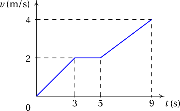
The figure shows the plot of the velocity of a body as a function of
time. Find the distance traveled from
to
s.
1 m
12 m
7 m
5 m
19 m
In a plot of the velocity as a function of position on the trajectory,
what does the slope of the curve represent?
The tangential acceleration.
The velocity.
The tangential acceleration divided by the velocity.
The product of the velocity and the tangential acceleration.
The velocity divided by the tangential acceleration.
Problems
The position of an object in its trajectory is given by the expression
(SI units). Determine the time, position and
tangential acceleration at all the instants when the object stops (its
velocity is
= 0).
The acceleration of object that moves along the
axis is
=
−4 m/s2. If at
= 0, the velocity is
= +24 m/s and the object is at the position
= 0, find its velocity
and position at
= 8 s and the total distance traveled by
the object from
= 0 to
= 8 s.
At
= 0 an object is at rest in the
position
= 5 cm in a path. From that moment,
the object starts to move in the positive direction of the
path, stopping again at
. The expression for the
tangential acceleration between
and
is
, where time is measured in
seconds and the acceleration in cm/s2. Find:
(a) The instant
when the object
stops. (b) The position along the path at that
instant.
The expression for the tangential
acceleration of a particle is
,
where
is a positive constant. The particle is
initially at rest at
= 800 mm and it starts
moving passing by
= 500 mm with a velocity
−6 m/s. Find: (a) The value of the
constant
. (b) The velocity of the particle at
= 250 mm.
The acceleration of an object that
oscillates on the
axis is
, where
is
a positive constant. Find:
The value that
must have so that
=
15 m/s at
= 0 and
= 0 at
=
3 m.
The velocity of the object at
= 2 m.
The tangential acceleration of an object
is
(SI units), where
is the position on the trajectory and
is a
constant. Knowing that the object crosses the origin
with velocity
= 17 m/s, find the velocity
at
= 4 m for each of the following values of the
constant: (a)
= 0, (b)
= 0.015,
(c)
= −0.015.
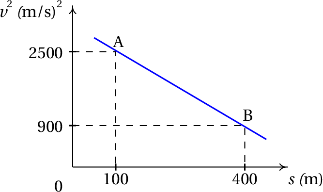
The square of the velocity
of an
object decreases linearly as a function of its position
on the trajectory, as shown in the figure. Compute the
distance traveled by the object during the last two
seconds before it reaches point B.
The tangential acceleration of an object
is
= −0.4 v, where
is measured in mm/s2 and
in
mm/s. Knowing that at
= 0 the velocity is
30 mm/s, find:
The distance traveled by the object from
= 0 until
it stops.
The time it took the object to travel that
distance.
The time
when the velocity of the object is 1
percent of the initial velocity at
= 0.
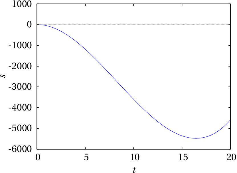
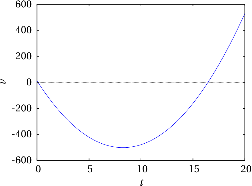
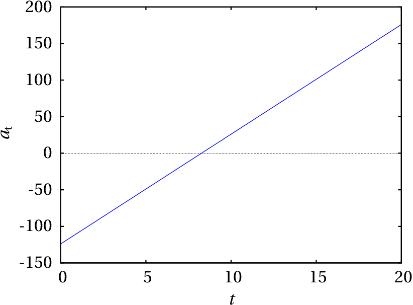
The position of a particle that moves
along the
axis is given approximately by the
expression
(SI
units).
Find the expressions for the velocity and the
acceleration as a function of time.
Find the values of the time, position and acceleration
in all the instants when the particle is as rest (
= 0).
Make the plots of position, velocity and acceleration
in the interval 0 ≤
≤ 20.
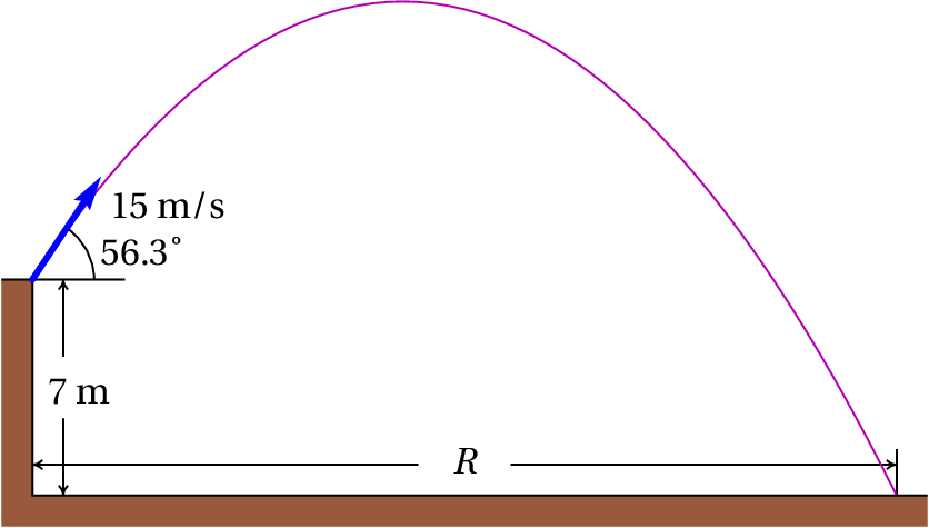
A projectile is thrown from the top of a
a building, 7 m above the ground, with a speed of
15 m/s in a direction 56.3° above the horizontal,
as shown in the figure. Assuming that the air resistance
can be neglected, find:
The time of flight, namely, the time interval since
the projectile is thrown until it hits the ground.
The horizontal range, namely, the distance
in
the figure.
A marble is thrown over the horizontal
surface on the top of some stairs, and it leaves the top
of the stairs with horizontal speed of 3 m/s. Each step
goes down 18 cm and is 30 cm wide. On which step
will the marble land?
The expression for the tangential
acceleration of an object falling freely through the air
is, including the air resistance,
, where
and
are constants. If the object
starts falling from rest at
= 0,
Prove that the velocity at any later time
is
Find the expression for the velocity of the object
after it has fallen a distance
.
Why is it that the velocity
is called terminal velocity?
Answers
Questions:1. A. 2. B. 3.
A. 4. C. 5. C.
Problems
= 0,
= 10 m,
=
−12 m/s2 and
= 2 s,
=
2 m,
=
12 m/s2.
Velocity −8 m/s, position
= 64 m and
distance traveled equal to 80 m.
(a) 3 s (b) 25.25 cm.
(a) 24 m3/s2
(b) 11.49 m/s.
(a) 25 s−2
(b) ±11.18 m/s (the object oscillates).
(a) ±15 m/s, because the object
oscillates. (b) ±14.74 m/s, because
the object oscillates. (c) 15.25 m/s, only
positive because the object moves always in the positive
direction. (To find out whether the object oscillates or
not, one can find the expression for
as a function
of
and look at its plot).
65.33 m
(a) 75 mm (b) infinite
(c) 11.51 s.
,
At
s,
m,
m/s2. Em
s,
m,
m/s2
The plots are the following
(a) 3.02 s. (b) 25.1 m.
On the fourth step.
(b)
(c) Because after a long time
approaches:
Correct
The increase of the velocity during the 3 seconds equals
the integral of
, with respect to time, which
should then be added to the initial velocity.
(click to continue)
Wrong
18 m/s is just the increase of the velocity during the 3
seconds. That increase must be added to the initial velocity.
(click to continue)
Wrong
The increase of the velocity during the 3 seconds equals
the integral of
, with respect to time, which
should then be added to the initial velocity.
(click to continue)
Wrong
The increase of the velocity during the 3 seconds is not
equal to
times
, but the integral
of
, with respect to time, from
= 0 to
= 3.
(click to continue)
Wrong
the velocity cannot remain constant because there is
tangential acceleration, always positive, which implies an
increase in the velocity.
(click to continue)
Wrong
Positive tangential acceleration implies increase of the velocity and since the velocity is positive it is then getting bigger and the object is speeding up.
(click to continue)
Correct
Positive tangential acceleration implies increase of the
velocity and since the velocity is negative its absolute
value is then getting smaller, so the object is slowing down.
(click to continue)
Wrong
It can be concluded that the absolute value of
is
getting bigger, but that doesn't give any information about
the velocity, because it might have other components, such
as
, that might be decreasing.
(click to continue)
Wrong
It can be concluded that the absolute value of
is
getting smaller, but that doesn't give any information
about the velocity, because it might have other components,
such as
, that might be increasing.
(click to continue)
Wrong
It can be concluded that the absolute value of
is
getting bigger, but that doesn't give any information about
the velocity, because it might have other components, such
as
, that might be decreasing.
(click to continue)
Correct
The derivative of
with respect to
is obtained by
multiplying its derivative with respect to
, times
itself (derivative of
with respect to
).
(click to continue)
Wrong
The acceleration
is the derivative of
with
respect to
, which is not equal to the derivative with
respect to
.
(click to continue)
Wrong
The acceleration
cannot be obtained dividing
by
. The equation
is
only valid when
is constant, which is not the case
here.
(click to continue)
Wrong
If you obtained this result dividing
by
,
that is not the correct way to compute the tangential
acceleration. If you found it as the derivative of the
velocity, you made an error in the differentiation.
(click to continue)
Wrong
If you obtained this result from the equation
, that equation is
only valid when the acceleration
is constant (not
true in this case) and the initial velocity
is zero
at
= 0 (that part is correct in this case).
(click to continue)
Wrong
The distance traveled is the integral of
, from
=
0 to
= 5, which in the plot corresponds to the area of
the triangle from
= 0 to
= 3, plus the area of the
square from
= 3 to
= 5.
(click to continue)
Wrong
The distance traveled is the integral of
, from
=
0 to
= 5, which in the plot corresponds to the area of
the triangle from
= 0 to
= 3, plus the area of the
square from
= 3 to
= 5.
(click to continue)
Correct
The distance traveled is the integral of
, from
=
0 to
= 5, which in the plot corresponds to the area of
the triangle from
= 0 to
= 3, plus the area of the
square from
= 3 to
= 5.
(click to continue)
Wrong
The distance traveled is the integral of
, from
=
0 to
= 5, which in the plot corresponds to the area of
the triangle from
= 0 to
= 3, plus the area of the
square from
= 3 to
= 5.
(click to continue)
Wrong
The distance traveled is the integral of
, from
=
0 to
= 5, which in the plot corresponds to the area of
the triangle from
= 0 to
= 3, plus the area of the
square from
= 3 to
= 5.
(click to continue)
Wrong
The slope of the plot represents the derivative
, which is not necessarily equal
to
.
(click to continue)
Wrong
The slope of the plot represents the derivative
, while the velocity is the
derivative
(click to continue)
Correct
The slope of the plot represents the derivative
, equal to
(click to continue)
Wrong
The slope of the plot represents the derivative
, with units of 1 over time, while
has units of distance squared over time
cubed.
(click to continue)
Wrong
The slope of the plot represents the derivative
, with units of 1 over time, while
has units of time.
The increase of the velocity during the 3 seconds equals the integral of , with respect to time, which should then be added to the initial velocity.
(click to continue)