Introduction
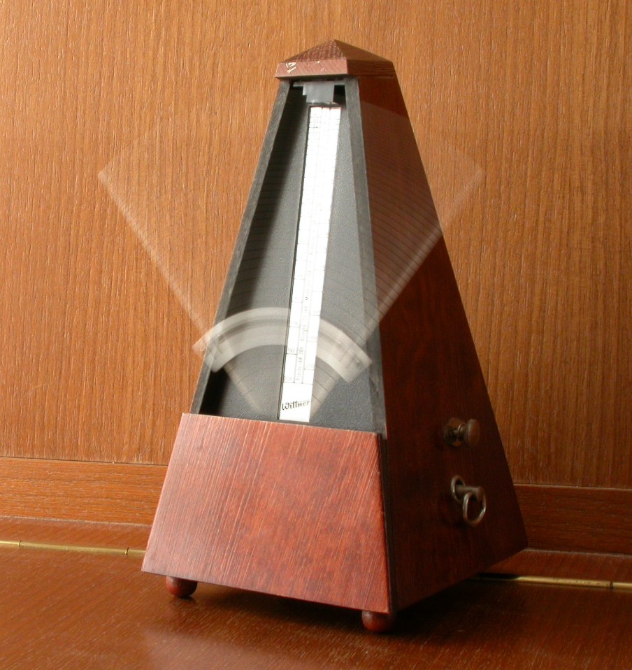
A metronome produces pulses of regular duration that can be adjusted by shifting a weight on the oscillating rod. Oscillators play a very important role in the theory of dynamical systems, as study cases for linear systems.
Jaime E. Villate. Dynamics and Dynamical Systems,
University of Porto, Portugal, 2019
A metronome produces pulses of regular duration that can be adjusted by shifting a weight on the oscillating rod. Oscillators play a very important role in the theory of dynamical systems, as study cases for linear systems.
A dynamic system with two state variables is defined by two evolution equations with the general form 7.2 introduced in Chapter 7:
It is said that the system is linear when the two functions and are linear combinations of the state variables:
where , , and are four constants.
The two evolution equations can be written more compactly using matrices:
The equilibrium points can be found by equating the term in the right of equation 9.3 to a matrix with zeros in the two lines, giving a homogeneous system of linear equations. A homogeneous system of linear equations always has at least one solution, called the trivial one, in which all variables are null. In some cases, when the determinant of the system matrix is zero, there are an infinite number of solutions. Therefore, if the determinant of the matrix is nonzero, the dynamical system has a single equilibrium point: , located at the origin of the phase space. In cases where the determinant of the matrix is zero, the derivatives of the two state variables are the same function, multiplied by a constant, and the system can be reduced to a linear system with a single state variable and a single equilibrium point at the origin.
When the evolution equations are linear combinations of the state variables plus a constant, the equilibrium point is no longer the origin of the phase space but it is possible to obtain a linear system by means of a change of variables, which corresponds to moving the origin to the equilibrium point, as done in the following example.
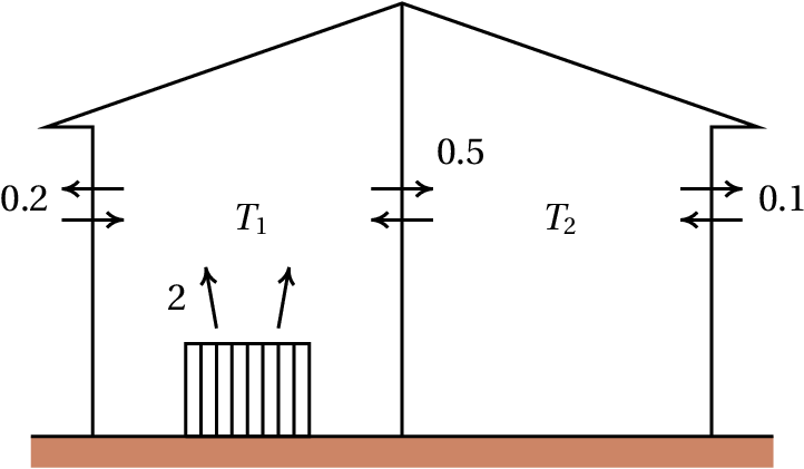
The heat transfer equations which determine the temperatures and in two rooms of a house, are the following:
where the temperatures are measured in degrees Celsius and the time in hours. The outside temperature is 8 °C. The terms and represent the heat coming from each room to the exterior per unit of time, divided by the heat capacities of each room. The term is related to the heat passing from one room to the other and the constant term 2 is due to the fact that in the first room a heater is providing a constant amount of heat every hour. Determine the temperatures of the two rooms once they reach constant values and rewrite the system as a linear one.
Resolution. The right-hand sides of the two differential equations define the phase velocity components in phase space ( , ). The equilibrium points, where the state of the system remains constant, are the points where those components are zero. Using the commandsolve of Maxima,
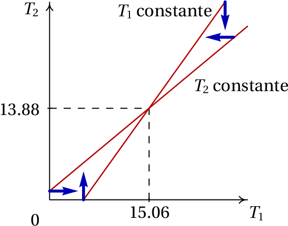
namely, the equilibrium temperatures of the two rooms are 15.06 °C and 13.88 °C.
To make the system linear, we move the coordinates origin to the equilibrium point. This is achieved by defining two new variables:
In terms of these new variables the evolution equations are similar to the original equations, but without the constant terms:
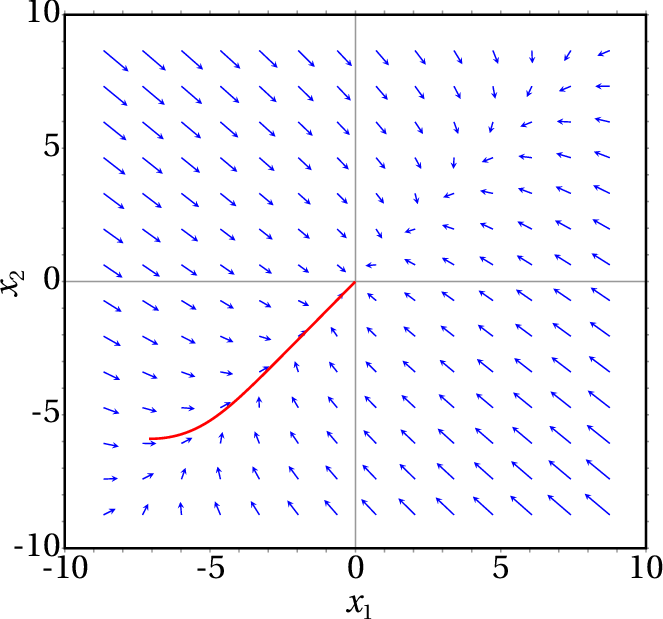
Figure 9.1 shows the nullclines for Example 9.1, which are the curves where each component of the phase velocity is zero. In the nullcline for , the derivative is zero and therefore, if the initial state was a point on this line, the temperature would remain constant at that initial instant and the state would evolve in the direction parallel to the axis. If the initial state was in the nullcline of , the sate would evolve in the direction parallel to the axis. The equilibrium point lies at the intersection of the two nullclines. In the region between the two nullclines, the vectors in the figure show that the phase velocity must point in the direction of the equilibrium point and the state should approach the equilibrium point; but what happens in the other regions? does the system evolve towards the equilibrium pint too? A general method for answering this question is introduced in the next section.
When the evolution equations are obtained from a single second order differential equation, , the dynamic system is linear if the function is a linear combination of and . In that case, the matrix form of the system is the following
where and are two constants.
In Example 9.1, if the temperatures of each room reach the equilibrium values, they will remain constant. But will the temperatures ever reach those values? Or will it happen that as the temperature of one of the rooms approaches its equilibrium value, the other temperature moves away from its equilibrium value? Also, if the initial temperatures are very close to their equilibrium values, will they get even closer to the equilibrium or will they get farther away from the equilibrium values?
In the systems discussed in Chapter 7, when the initial state of the system is near an unstable equilibrium point, the system may end moving to infinity, or depart initially and then return to the initial point. If the initial state is near a stable equilibrium point, the system oscillates. In Example 9.1, if there were cycles in phase space, it would be possible that the two temperatures fluctuated indefinitely, without ever stabilizing.
We are going to introduce a general method to analyze the stability of linear systems, namely, their behavior in the vicinity of the equilibrium points. The matrix equation 9.3 can be interpreted as the matrix representation of the vector equation:
where the position and the velocity of the state are vectors in phase space and is a linear operator acting on vectors of phase space producing other vectors in that space.
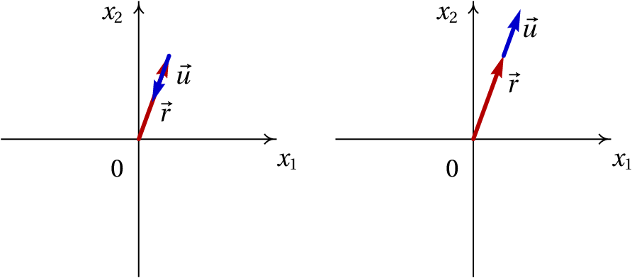
If at a given instant the phase velocity and the position vector in phase space, , are in the same direction, there are two possibilities as shown in Figure 9.2: if the two vectors are opposite, the state approaches the origin (equilibrium point) and if they point to the same side, the state departs from the origin. The condition for and to have the same direction is:
where is a real number. If is positive, the system will move away from the equilibrium point and if is negative, the system will approach the equilibrium point. Substituting the previous expression into equation 9.6 leads to:
The vectors satisfying equation 9.8 are called eigenvectors of th eoperator and the corresponding values are the operator's eigenvalues.
Find the eigenvalues and eigenvectors of the linear system of Example 9.1.
Resolution. Since the evolution equations have already been stored in the variables eq1 and eq2, we can use the command coefmatrix to obtain the system matrix (equation 9.4):
which are the same 4 coefficients of the linear combinations in equations 9.4. The command eigenvectors of Maxima gives the eigenvalues and eigenvectors of a matrix:
The first list shows the eigenvalues, and . The second list are the "multiplicities" of each eigenvalue, which in this case are both 1. The last two lists define the directions of the eigenvectors corresponding to the two eigenvalues; any vectors in the same direction of one of these two vectors, is also eigenvector.
Since there are two negative eigenvalues, there are two directions in the phase plane in which the state of the system approaches the equilibrium state at the origin. We can construct the phase portrait of the system using plotdf:
The syntax A[i] is used to obtain the th line of the matrix and the dot indicates matrix product. Figure 9.3 shows the phase portrait.
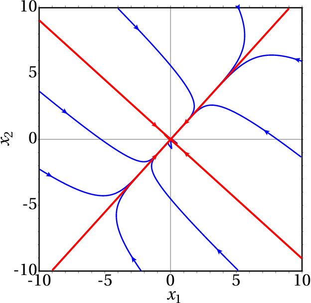
The directions of the two eigenvectors (the two lines) are plotted by entering the coordinates of the eigenvectors obtained in the result (%o7) into the field "Trajectory at"" in the configuration menu and then entering the same coordinates with opposite signs. If the initial state is not on one of the directions of the eigenvectors, the evolution curve approaches the direction of the eigenvector with the smallest eigenvalue in absolute value.
It should be noted that the two nullclines shown in Figure 9.1 are on both sides of the line with positive slope in Figure 9.3 and intersect at the origin, where the equilibrium point was displaced.
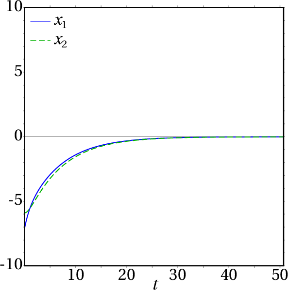
If the initial temperatures in the rooms were equal to the outside temperature, , then the initial values of the variables and would be 8−15.06 and 8−13.88. The evolution curve in phase space and the temperatures as a function of time can be plotted with the following command:
The result is shown in Figure 9.4. The plots of the time functions show that after 30 hours, the two temperatures reach practically the equilibrium values.
The general form of a linear dynamical system, with any state variables, is:
where is the state of the system in a vector space with dimensions and is a linear operator in that space. In a phase space with two state variables and , the matrix representation of equation 9.9 is equation 9.3.
If the determinant of the matrix is nonzero, there is a single equilibrium point at the origin: . The existence of eigenvalues of matrix implies the existence of directions in which the state approaches or departs in a straight line from the equilibrium point. The eigenvalues of matrix are the numbers that satisfy equation 9.8. In a phase space with two variables, this equation leads to:
That determinant leads to the following quadratic equation, called characteristic equation :
where is the trace of the matrix and its determinant. The two roots of the characteristic equation are:
If the roots are complex numbers, it means that there are no eigenvectors in the phase plane ( , ). If there is a single real root, there will be at least one eigenvector and if there are two different real roots, there will be two independent vectors linearly independent in phase space.
When the determinant is negative, the expression inside the square root in equation 9.12 is positive and
This implies that there are two real eigenvalues, and , one positive and the other negative.
These two eigenvalues correspond to two linearly independent eigenvectors, which define two directions in the phase plane where the system evolves along a straight line (see Figure 9.5). In the direction corresponding to the negative eigenvalue, the negative sign implies that there are two evolution curves which are straight lines approaching the origin. In the direction associated to the positive eigenvalue, the positive sign implies two evolution curves which are straight lines moving away from the origin.
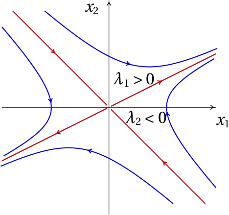
The other evolution curves of the system are curves that approach the origin for some time, but always end up moving away to infinity (Figure 9.5). This type of equilibrium point is called saddle point. Saddle points are unstable equilibrium points.
Notice that even though there are two evolution curves that start on the saddle point and two evolution curves that approach it, there can be no homoclinic orbits starting and ending at that point, because those evolution curves are straight lines that extend to infinity. Linear systems can never have homoclinic orbits. They never have heteroclinic orbits either, because there should be two ore more equilibrium points in a heteroclinic orbit, but linear systems have only one equilibrium point.
When the determinant is positive but less than , there are two real solutions of equation 9.12 both with the same sign of .
If the two eigenvalues are negative, there are two directions in the phase space in which the state approaches the equilibrium point (left side of Figure 9.6). Due to the continuity of the evolution curves, any other evolution curve will be a curve approaching the equilibrium point. The equilibrium point in this case is called a stable node or attractive node.
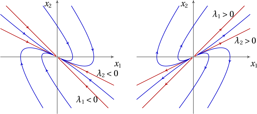
If the two eigenvalues are positive, there are two directions in phase space where the state moves away from the equilibrium point. Whatever the initial state, the system always moves away from the equilibrium point (right side of Figure 9.6) and the point is called an unstable node or repulsive node.
When the determinant is greater than , the two solutions in equation 9.12 are complex numbers . This means that there are no straight-line evolution curves. All evolution curves are curved.
The sign of the real part of the complex solutions of equation 9.12 determines whether the evolution curves approach the equilibrium point or move away from it. If the real part of the roots is negative (matrix with negative trace), the evolution curves are spirals that approach the equilibrium point, as in the leftand side of figure 9.7 and the equilibrium point is called stable focus or attractive focus.
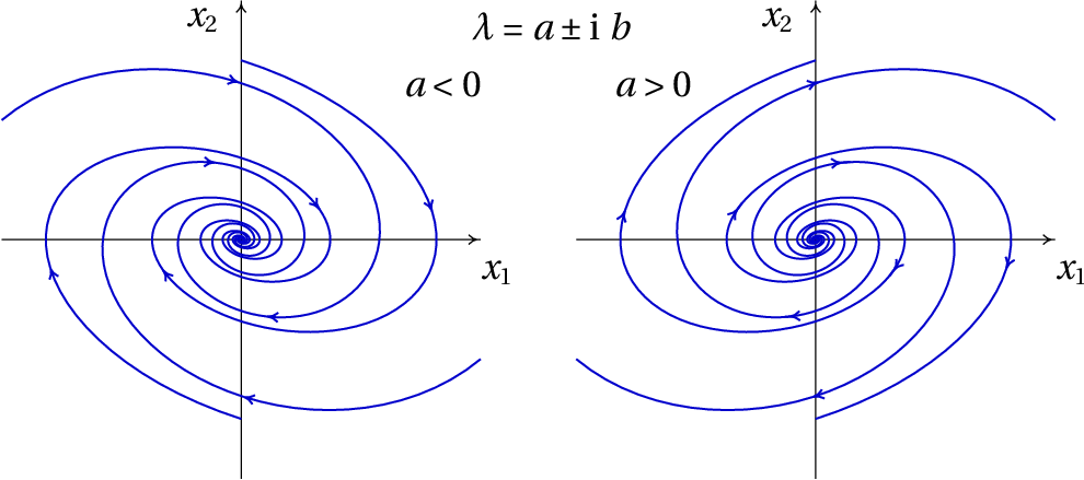
If the real part of the roots is positive (matrix with positive trace), the evolution curves are spirals moving away from the equilibrium point, as in the right-hand side of Figure 9.7) and the equilibrium point is called unstable focus or repulsive focus.
If the trace of the matrix is zero, the solutions of equation 9.12 are two purely imaginary numbers, with the same imaginary part but with opposite signs. In that case all evolution curves are cycles; the of equilibrium point is stable and it is called center.
Figure 9.8 shows a summary of the different types of equilibrium points, in terms of the trace and the determinant of the system matrix.
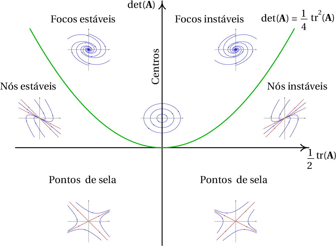
When the determinant is equal to , which corresponds to the points in the parabola in figure 9.8, there is only a real eigenvalue.
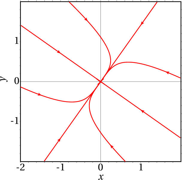
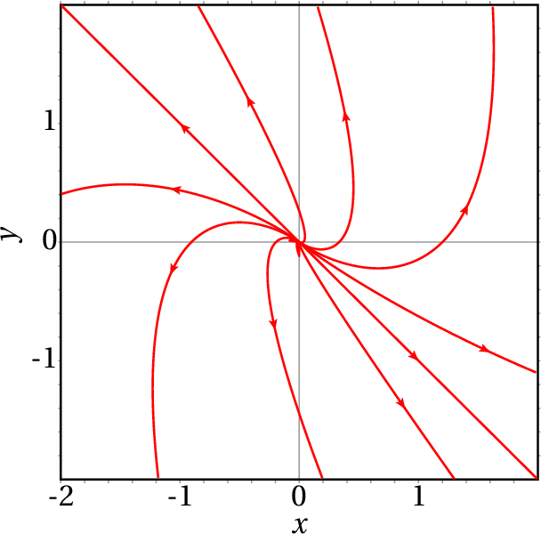
In that case the equilibrium point may be either one of two types. If the matrix is diagonal, the two elements in the diagonal are both equal to the eigenvalue and any vector in phase space is an eigenvector of the matrix. This implies that all evolution curves are straight lines, starting at the origin if the eigenvalue is positive, as in the left-hand side of figure 9.9, or ending at the origin if the eigenvalue is negative. The equilibrium point is called proper node; it is either stable or unstable, depending on the sign of the eigenvalue.
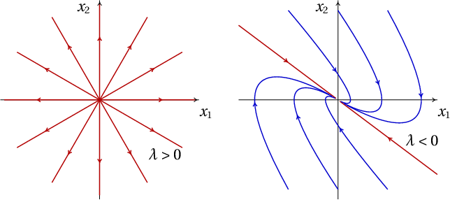
In the second case, when the matrix is not diagonal, there is only one straight-line in the phase portrait and the equilibrium point is called improper node. If the eigenvalue is negative, the improper node is stable, as in the right-hand side of Figure 9.9) and if the eigenvalue is positive the equilibrium point is an unstable improper node. If the improper node is unstable, the evolution curves start from the origin in two opposite directions; the curves starting in one of the directions curve to one side and the others curve in to the other side. If the improper node is stable, the evolution curves have a similar shape but in evolve in the opposite direction.
A convenient way to identify type of equilibrium of a linear system is as follows: if the matrix is diagonal, the diagonal elements are the eigenvalues. If the two eigenvalues in the diagonal are equal, the point is a proper node, unstable if the eigenvalue is positive or stable if the eigenvalue is negative; in this case any vector in phase space is an eigenvector.
If the matrix is not diagonal, we write its characteristic equation 9.11 and find the eigenvalues. Table 9.1 can the be used to classify the equilibrium point, according to the type of eigenvalues found.
| Eigenvalues λ | Type of point | Stability |
|---|---|---|
| 2 real numbers with opposite signs | saddle point | unstable |
| 2 real positive numbers | repulsive node | unstable |
| 2 real negative numbers | attractive node | stable |
| 2 complex numbers with positive real part | repulsive focus | unstable |
| 2 complex numbers with negative real part | attractive focus | stable |
| 2 imaginary numbers | center | stable |
| 1 real positive number | repulsive improper node | unstable |
| 1 real negative number | attractive improper node | stable |
When a system is linear and conservative, the condition 7.14 that the divergence is null implies, using the notation of equations 9.2,
namely, the trace of the system matrix, , is equal to zero, and we can conclude from Figure 9.8, that the equilibrium point at the origin must be a center, if it is stable, or a saddle point, if it is unstable. Conservative linear systems never have nodes or foci.
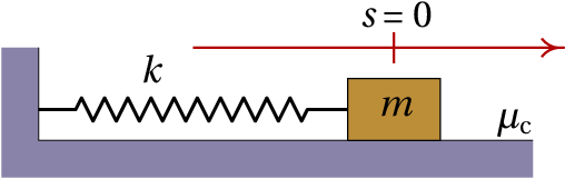
In mechanical systems with a single degree of freedom , when the equation of motion is a linear combination of and , it leads to a linear dynamical system. Therefore, the equation of motion of linear conservative systems has the general form:
where and are constants. The term is the tangential component of the conservative force, divided by the mass ; and the term is the tangential component of the non-conservative force, divided by .
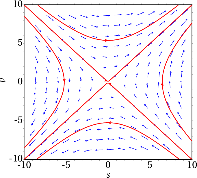
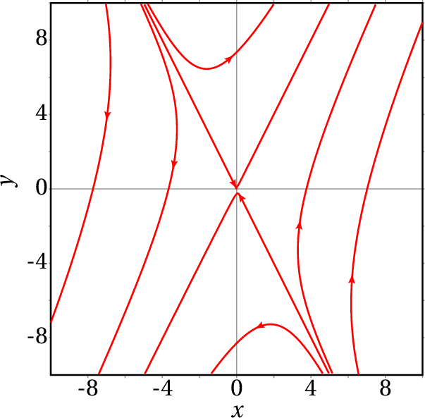
An inverted oscillator is a system with equation of motion: , where is a positive constant. Analyze the stability of the system and plot the phase portrait in some system of units that make .
Resolution. The state variables are and and the matrix form of the evolution equations (equation 9.5) is:
The trace of the matrix is null and its determinant is equal to , which is negative. Thus, the characteristic equation is and the eigenvalues are and . According to table 9.1, the equilibrium point at the origin is a saddle point (unstable).
The phase portrait for can be done with the command:
Figure 9.10 shows the graph obtained after tracing some trajectories.
Analyze the stability and evolution curves of a simple harmonic oscillator.
Resolution. The simple harmonic oscillator was discussed in section 6.4, where its equation of motion was derived (equation 6.31 ):
where is a positive constant.
Therefore, the matrix form of the system is:
The trace of the matrix is zero and its determinant is , which is positive. Consequently, the eigenvalues are two purely imaginary numbers:
and the equilibrium point is a center.
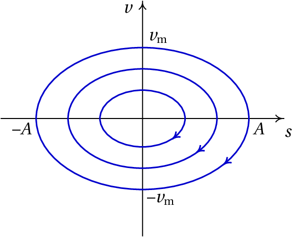
If the initial state of the oscillator is the equilibrium state, , it will remain at rest; otherwise, the evolution curve will be an ellipse (Figure 9.11), which corresponds to a simple harmonic motion with angular frequency . That is, whenever the eigenvalues of a linear system of two variables are purely imaginary, the system is a simple harmonic oscillator, with angular frequency equal to the modulus of the eigenvalues, |. In the case of a body of mass attached to a spring with elastic constant , the constant is and the angular frequency is .
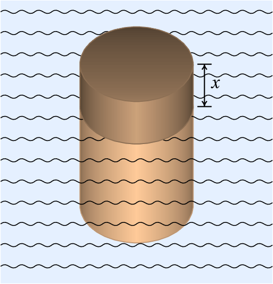
The simple harmonic oscillator of Example 9.4 is an idealized system, since in practice there are dissipative forces. An example is the suspension system in an car (Figure 9.12). Each wheel is attached to the body by means of an elastic spring; inside each spring there is a cylinder (shock absorber) with a piston that moves in oil.
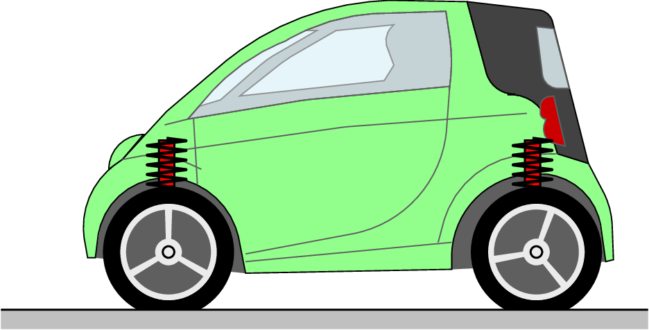
Let be the height of the point of the body where the spring is supported, measured from the equilibrium position ; the total vertical force exerted by the shock absorber on the body is:
where and are positive constants; is the spring's spring constant and depends on the size of the piston and the viscosity coefficient of the oil inside the cylinder.
This force leads to the following linear system:
where is the angular frequency, , and equals .
The trace of the system matrix is , negative, and the determinant is , positive. Thus, the eigenvalues are either negative real numbers or complex numbers with negative real part. This implies that the system is always stable, eventually ending at the equilibrium state and .
However, the way the system approaches the equilibrium point will depend on the type of point. The damping is called weak when,
and in that case the eigenvalues are complex; the system matrix is in the region of stable foci in Figure 9.8. The evolution of as a function of time is an oscillatory function with decreasing amplitude, as shown in Figure 9.13.
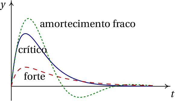
In the case when:
we say that there is critical damping. In this case there is a single real eigenvalue. Since the matrix is not diagonal, the equilibrium point is a stable improper node. The evolution of in terms of is shown in Figure 9.13.
Finally, the damping is called strong if:
there are two different negative eigenvalues. The equilibrium point is a stable node and approaches the equilibrium point faster than in the other two cases (Figure 9.13).
The suspension system should ensure that the car approaches the equilibrium immediately, without oscillations which could have bad consequences for the car stability. Thus, the shock absorbers should provide strong damping, making the equilibrium point a node.
After some use, dirt and the impurities in the shock absorber's oil reduce its viscosity diminishes; some oil might also leak out. These factors reduce the value of the constant below its critical value. If, by pushing the car body down, the car swings slightly, it is time to replace the shock absorbers.
(To check your answer, click on it.)
 Being the maximum height reached by the ball
m and the maximum deformation of the ball on the floor
cm, compute:
Being the maximum height reached by the ball
m and the maximum deformation of the ball on the floor
cm, compute:
Questions: 1. E. 2. E. 3. B. 4. B. 5. A.
Problems
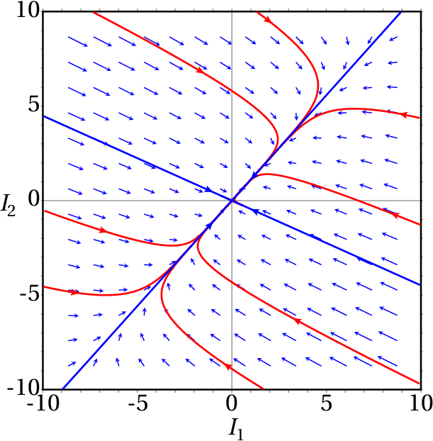 (d) Saddle point. It can not describe a real
transformer, because the instability of the system
implies that with finite initial currents the currents
would increase to infinity, which is not
possible.
(d) Saddle point. It can not describe a real
transformer, because the instability of the system
implies that with finite initial currents the currents
would increase to infinity, which is not
possible.
(click to continue)
(click to continue)
(click to continue)
(click to continue)
(click to continue)
(click to continue)
(click to continue)
(click to continue)
(click to continue)
(click to continue)
(click to continue)
(click to continue)
(click to continue)
(click to continue)
(click to continue)
(click to continue)
(click to continue)
(click to continue)
(click to continue)
(click to continue)
(click to continue)
(click to continue)
(click to continue)
(click to continue)
(click to continue)