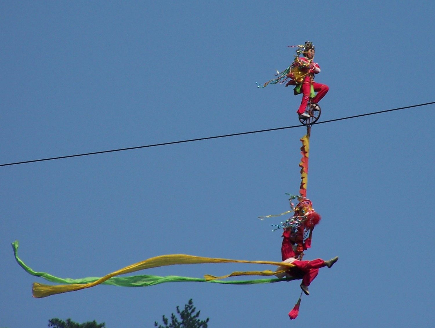
To analyze a dynamical system, it is important to determine the
existence of equilibrium points. The acrobats in the photograph are in
a stable equilibrium position: if the bicycle tilts laterally, the
weight of the acrobat hanging underneath causes the system to tilt in
the opposite direction, returning to the equilibrium position. If the
acrobat on the bike did not have the second acrobat hanging, that
equilibrium position would be unstable: if the bicycle tilted
sideways, its weight plus that of the acrobat would make them tilt
further, moving the bicycle away from the equilibrium position.
7.1. Differential equations
The kinematic equations are ordinary equations differential. An ordinary
differential equation —or ODE for short— is any expression
that relates a function, for example
and its derivatives:
,
, etc. For example:
;
in this case the independent variable is
and the dependent
variable is
, which depends on
. Many problems of science and
engineering lead to ordinary differential equations that need to be
solved to find the dependent variable in terms of the independent
variable. There are equations that appear in several different areas;
for example, the equation of the simple harmonic oscillator, analyzed
in chapter 6, is of the general form
, where
is a
positive constant. In the various scientific areas in which similar
equations appear, the behavior of the system can be analyzed by
analogy with the movement of a body connected to an elastic
spring.
7.1.1. First order equations
An ODE is of first order if the only derivative that appears in the
equation is the first-order derivative. If the independent variable is
and the dependent variable
, these types of equations can be
written in the general form
(7.1)
where
is an expression of
and
. All the
differential equations that were solved in chapter 1 by the method of
separation of variables are of this type. But there are other
first-order equations that can not be solved by this method. For
example, the equation
can not be separated into a
term that depends only on
and anotherr that depends only on
.
An ODE admits many different solutions, depending on the initial
values (
,
). In the examples solved in chapter 1, different
solutions were obtained for different integration limits.
A first-order ODE with the general form
is
called autonomous
because the independent variable
does not appear explicitly on the
right-hand side. In this case, the solution
is still a function of
time but it turns out that the functions obtained with the initial
conditions (
,
), (
,
), (
,
), etc. are
the same function but displaced along the axis of
. It is then said
that the way the system evolves from the initial value
is the
same regardless of when the system starts to evolve.
In physical terms, an autonomous system is a system that is always
governed by the same physical laws. For instance, the height
of
a body in free fall from a point with height
always decreases in
the same way, as long as the value of
doesn't change.
7.2. Systems of autonomous differential equations
Consider now the case where there are two independent functions
and
, which depend on time and are defined by two
first-order autonomous differential equations:
(7.2)
For example, the system:
(7.3)
We intend to find the functions
and
from the
known values of
and
in an initial instant
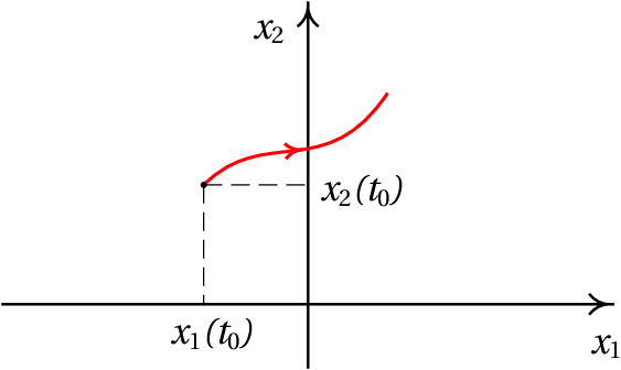
. We can visualize the problem on a graph where
and
are in two perpendicular axes, as in
figure 7.1. Two initial values
and
, at an initial instant
, define a point in that plane
and in the following instants the values of
and
will
change, causing that point to move along a curve on that plane.
Figure 7.1: Phase space of an autonomous system with two variables.
The plane with the axes
and
is
called phase
space and at every instant
, the point of phase space
defined by the coordinates (
,
) represents
the state of the system
at that instant. The two variables
and
are
the state
variables and the curve represented in
figure 7.1, which shows the variation of
the state variables from an initial state, is called an evolution
curve of the system.
Any point of phase space can be the initial state of the system
(
,
). The values of
and
at that point are well defined and determine how the
state variables
and
change in that point. The expression
, derivative of
with respect to time, gives the increase of
per unit of time. That is, the displacement of the projection of
the state of the system in the axis
per unit of time;
analogously,
gives the displacement of the projection of the
state of the system in the axis
per unit of time.
Therefore, the vector:
(7.4)
defines the displacement of the state of the system in phase space
per unit of time and is thus called phase velocity. The
differential equations 7.2 are
called evolution equations of the system, and their right-hand
sides define the phase velocity at any point in phase space. For
example, the expression for the phase velocity of the system with
evolution equations 7.3 is:
The initial state (
,
) in the instant
moves in the phase space with phase velocity
. At a
later time
, the phase velocity
may be another
different vector that makes the state move in a different direction
and with a different speed. Thus, the evolution of the state of the
system as a function of time is defined by a continuous curve in phase
space, passing through the initial state (
,
). Through each point of phase space where functions
and
are defined passes one, and only one, evolution curve of the
system.
The phase velocity
is tangent to the evolution
curves. Two different evolution curves can never crossed each other,
because at the point of intersection there would be two different
phase velocities, which is not possible.
7.2.1. Direction fields
It is possible to have an idea of how a dynamical system evolves in
time, without having to solve the differential
equations 7.2.
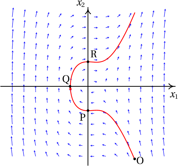
Figure 7.2 shows the direction of the
phase velocity at various points in the phase space, for a concrete
example. This type of graph is called a
direction field.
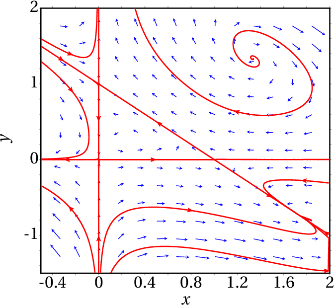
Figure 7.2: Direction field of a dynamical system
and an evolution curve.
We can predict how the evolution curve will be from an initial
state in an instant
by looking at the direction field. For
example, figure 7.2 shows one of the possible
evolution curves of the system, from the initial state P, with
and
. It is also possible to see the previous evolution of
the system in
which led him to reach the state P in
. The figure shows that the system passed state O before reaching
state P.
Along the evolution curve,
decreases from its initial
positive value in
to negative values, reaching a minimum value;
it then increases and becomes positive again. The variable
increases from its initial negative value and when
is
approaching zero, it decreases slightly and increases again while
remains negative.
7.2.2. Second order differential equations
The general form of a second-order autonomous differential equation
is:
(7.5)
Which can be reduced to two evolution equations of a dynamical
system with two state variables. We just have to consider the first
derivative
as another variable state variable
, which
also depends on time; therefore, the second derivative
is
the same as
and the differential equation can be written as
, which is a first-order equation. But as this new
equation has two state variables, a second equation is needed which is
the definition of the new state variable:
. Thus, the
initial equation is equivalent to the system of two equations:
(7.6)
These two equations define a dynamical system with state variables
and
. The expression of the phase velocity is:
(7.7)
In mechanical systems, Newton's leads to the expression for the
acceleration, called equation of motion. Since the acceleration is the
second derivative of the position, the equation of motion is a
second-order differential equation. The velocity — first
derivative of the position — is the additional state variable
that reduces the equation of motion to two first-order differential
equations. The state of the system at each instant is given by its the
position and velocity.
Example 7.1
A 0.5 kg object moves along a curve, under the action of a force
with tangential component
(in SI
units), where
is the position along the curve. (a) Write
the evolution equations of the system and identify the state
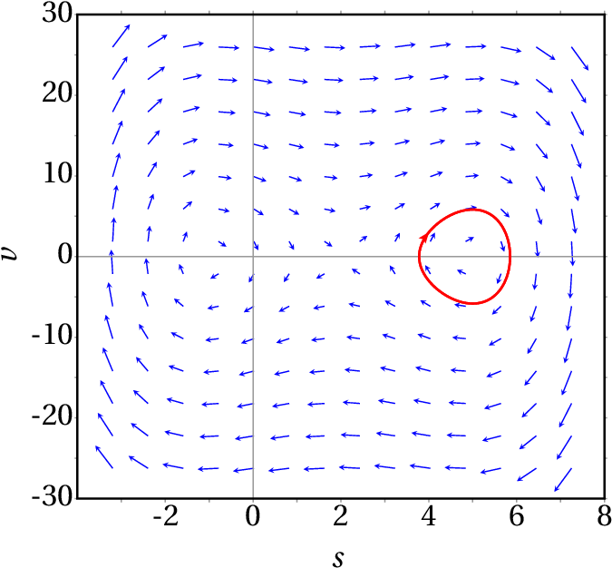
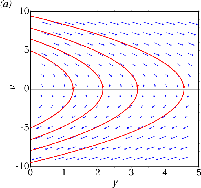
variables. (b) Plot the direction field for values of
in
the interval [-4, 8] and values of
in the interval [-30,
30]. (c) At an initial instant the particle is in the position
, with speed
m/s; plot the evolution curve of the
particle in phase space.
Solution. (a) The tangential acceleration
is equal to the tangential component of the force, divided by the
mass:
This equation of motion is equivalent to the following two
equations of evolution of a dynamical system:
The state variables are the position along the trajectory,
, and
the velocity
.
(b) and (c) The phase velocity is the vector:
In Maxima, a direction field can be shown with the program
plotdf. The
first two arguments that should be given to the program are a list
with the components of the phase velocity and another list with the
names of the state variables. After that, the domain of the state
variables can be defined as shown below. To plot the evolution curve
that passes through the initial state
and
, the
option trajectory_at
is used:
The vectors representing the phase velocity were not drawn to their
true length, to prevent them from intersecting, but were adjusted to
be slightly smaller than the distance between the grid points on which
the vectors are drawn.
The evolution curve of the particle from
shows that the
particle is moving in the direction in which
increases,
accelerating to a maximum speed approximately
. It then slows
down until it stops (
), at approximately
. It then
accelerates again, but now in the sense that
decreases (
)
to a minimum speed approximately
, until it stops again near
. At this point the cycle is repeated indefinitely.
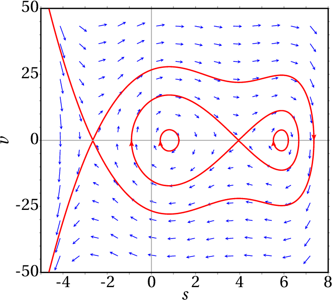
7.2.3. Phase portraits
The direction field provides a lot of important information about
the system. In the example shown in figure 7.3,
the initial conditions given lead to an oscillatory movement around
. The figure also shows that if the initial velocity were
greater, or if the particle started from
, the oscillation
would be up to values of
less than -1.5. It can also be seen that
there are other oscillations (closed evolution curves) around
.
A more complete graph, showing various evolution curves
that help describe the possible types of motion, is called
phase portrait
of the system.
The direction field is also useful to explain how the numerical
methods used to solve differential equations work. Given an initial
point in phase space and expressions that define the phase velocity at
each point in phase space, a sequence of points is created in which
each point follows the previous one in the direction defined by the
mean phase velocity between those two points. The
option trajectory_at of the
program plotdf, which was used
in the above example, causes the system of differential equations to
be solved numerically with initial conditions equal to the values
given and the solution is represented in the same graph of the
direction field.
As already mentioned, the first argument to be given to the
program plotdf must be a list
with the expressions that define the two components of the phase
velocity, that is, the derivatives of the two state variables. Each of
these expressions may depend solely on the two state
variables. Following this list there must be another list with the
names of the two state variables, in the same order that was used to
write their derivatives in the first list. There are several
additional options that can be used; the complete list can be found in
the chapter on numerical methods in the Maxima manual.
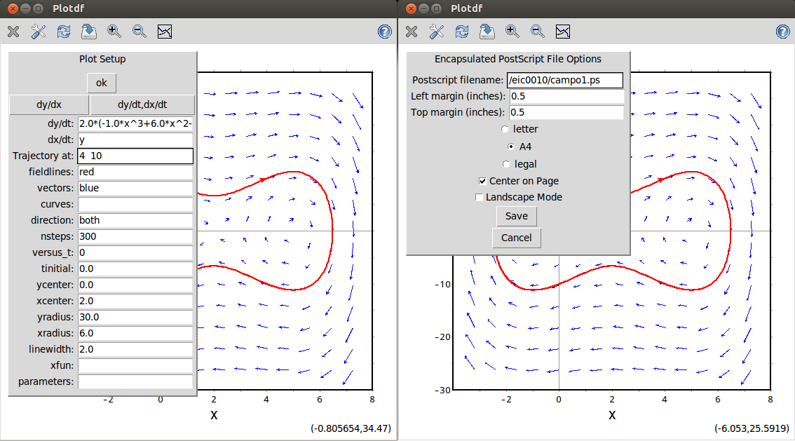
The program plotdf opens a
new window with the direction field, as shown in
figure 7.4. When the mouse is moved over
phase space, the coordinates of the pointer point appear in the lower
right corner. By clicking on the first mouse button on a point in the
graph, the evolution curve that passes through this point appears with
an arrow indicating the direction of evolution.
Figure 7.4: Config
and Save menus of the plotdf program.
The menu bar of the graphics window includes several buttons. The
buttons with the + and − signs are used to increase or decrease
the size of the graph. The button with a disk is used to save the
graph to a Postscript file. The button on the right, with a small
graph, opens a new window showing the plots of the two state variables
in terms of time, corresponding to the last evolution curve that has
been drawn.
The button with a screwdriver opens the "Plot SetUp" menu
(figure 7.4) which shows several
parameters that can be changed: the equations defining the phase
velocity components, the colors used for the phase velocity vectors
(vectors) and the evolution
curves (fieldlines), the domain,
etc.
If the vectors field is left blank, the
direction field vectors are not plotted and if the
fieldfieldlines is blank, no
evolution curves are drawn. When a parameter is changed, one must
select "ok" and then "Replot" (button with rotating arrows) to update
the graph.
The field called
direction has,
by default, the
value both, which means that
when one clicks on a point, the evolution curve through that point
will be plotted, extending for some interval of time after that point
and some interval of time before it. Changing this field to
forward
or backward,
the curve will shown only for some time interval after or
before the initial instant. Entering two coordinates in the
field called Trajectory at,
separated by space, and pressing the Enter key,
another evolution curve will be shown, passing through the
point with those coordinates.
7.3. Equilibrium points
At each point in phase space, the phase velocity indicates the
direction of the tangent to the evolution curve that goes through this
point. At points where the phase velocity is zero, there is no curve
passing through them. In those cases the state of the particle remains
constant. Those points are called equilibrium points.
Example 7.2.
Find the equilibrium points of the dynamical system
Solution. Since they are going to be used in several commands,
let us start by saving the two expressions on the right-hand side of
the evolution equations into two variables
(%i2)f1:4-x1^2-4*x2^2$ (%i3)f2: x2^2-x1^2+1$
We then use the command
solve
to find the equilibrium points, where the two expressions are equal to
zero
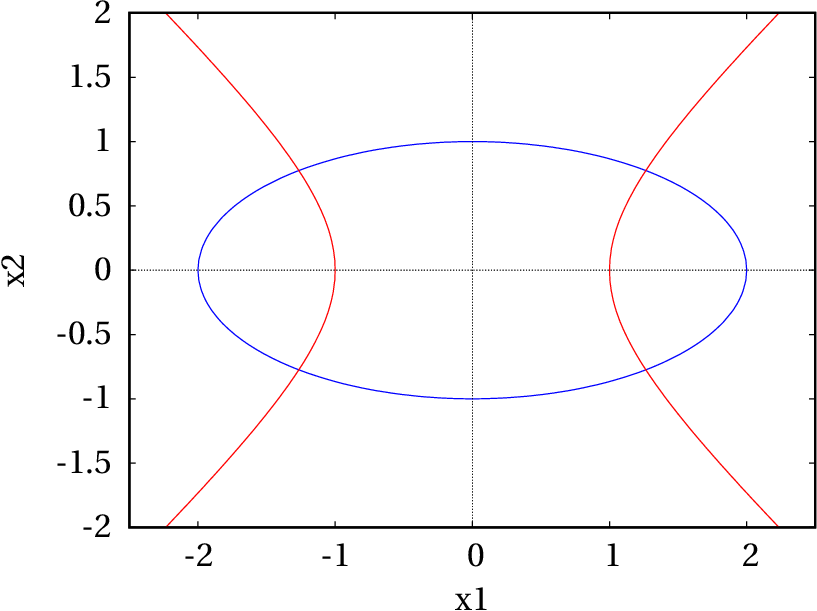
The curve where
vanishes is called nullcline for the variable
and in
this case it is the ellipse
. The nullclines for
are the two parts of the hyperbola
.
The equilibrium points of the system are the four points of
intersection between the nullclines of
and
. The plots of
these two curves can be obtained using Maxima's syntax for implicit
functions (in versions previous to 5.45, it was necessary to use the
program implicit_plot):
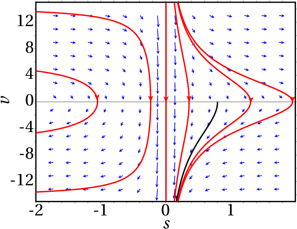
The result is shown in
figure 7.5. Inside the ellipse,
is positive, so the phase velocity points to the
right. Outside the ellipse the phase velocity points to the left. In
the region to the left of the hyperbola, the phase velocity points
downward, between the two branches of the hyperbola it points upward
and to the right of the hyperbola it points downward.
In mechanical systems where the two state variables are the
position
along the trajectory and the velocity
, if the two
components of the phase velocity are zero then the velocity and the
tangential acceleration are zero. This implies that the system is in a
state of static
equilibrium, in which the object remains at rest. In those
systems, all points on the
axis in phase space correspond to
states of rest (
), but not necessarily equilibrium states
(
). The equilibrium states of those dynamical systems
are the static equilibrium points, which are all on the
axis,
where
, and in with
also equal to zero.
At the points of the
axis where the phase velocity is not zero,
the system becomes at rest just for an instant, resuming its motion
immediately.
A kinetic
equilibrium state is a state in which the tangential
acceleration is zero but the object moves with constant velocity. In
the phase portrait those kinetic equilibrium states are straight lines
parallel to the
axis.
Example 7.3
An object with mass 0.3 kg moves under the action of a force with
tangential component (SI units):
where
is the position along the trajectory. (a) Find the
equilibrium points of the system. (b) Plot the phase portrait
of the system.
Resolution. (a) One can start by saving the
expression of the force in terms of
:
(%i7)Ft: -s^4/2 + 4*s^3 - 3*s^2/2 - 32*s + 25$
To find the equilibrium points, where the tangential force is zero,
we can use the command realroots, since we are only interested in the
real roots
(%i8)se: float (realroots (Ft));
(%o8)
There are then 4 equilibrium points, all with
And with the 4
values of
shown in (%o8). (b) In
order to plot the phase portrait we chose a domain in which the four
equilibrium points are visible and distinguishable:
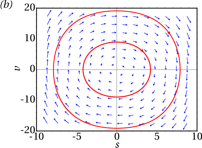
The evolution curves in the vicinity of the 2 equilibrium points in
and
are closed, with the equilibrium point inside
them. At the other two equilibrium points,
and
,
there are evolution curves that begin or end at the point (they
approach asymptotically to the point in the limits
or
). These types of curves
will be analyzed in more detail in the next two sections.
7.3.1 Stable and unstable equilibrium
The equilibrium points in
and
in
example 7.3
are stable
equilibrium points, because if the initial state of the
system is close to one of those points, the system will return to that
initial state.
The other two equilibrium points, at
and
,
are unstable
equilibrium points, because if the initial state of the
system is close to one of those points, the system will move farther
away from the equilibrium point.
The components of the phase velocity allows us to find the
equilibrium points. In the case of mechanical systems, with state
variables
and
, it is enough to find the roots of the
expression for tangential force (or tangential acceleration), with
respect to the position
, substituting
. In those systems the
expression for
or
, with
, can also
be used to classify the equilibrium points as stable or
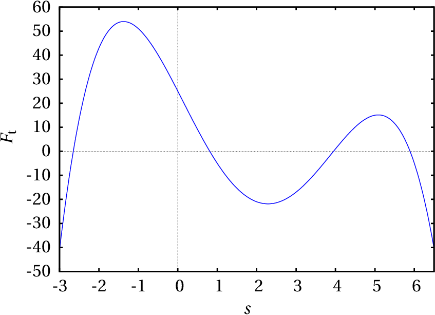
unstable. Figure 7.7 shows the plot of
the tangential force in example 7.3.
The equilibrium points
are the points in
figure 7.7 where the curve crosses the
axis. If at those points
crosses from a negative
value to a positive value, on the left of the point, where
, the force points to the left making
decrease, that
is, making the system move away from the equilibrium point. On the
right of the point, where
, the force is to the
right, making
increase, so the system also moves away from
equilibrium point. Thus, at those points the equilibrium is
unstable.
At the equilibrium points where
changes sign from
positive to negative, the force makes
increase if
, or decrease if
. Therefore, those
are stable equilibrium points.
In chapters 9
and 10 a more general
method to analyze the stability of the equilibrium points
will be introduced. The phase portrait also helps to
analyze the stability of the equilibrium points.
7.3.2. Cycles and orbits
In example 7.3
(figure 7.8) the evolution curves in the
vicinity of the stable equilibrium points,
and
,
are closed curves around the equilibrium point. Each of those closed
curves, called cycles,
imply oscillatory motion around the equilibrium point.
A cycle is a closed curve in phase space that corresponds to a
periodic oscillation of the state variables.
Figure 7.8: Phase portrait of the system of example
7.3 .
Figure 7.8 shows the important parts in the
phase portrait of the example in
figure 7.6. At the unstable equilibrium
point
there are two evolution curves that approach
asymptotically that point at both limits
and
; one on the left and one on the right. Neither
of those two curves is really a closed curve because the equilibrium
point itself is not part of any of those curves. Each of those two
curves is called a homoclinic orbit and they correspond to
a soliton: a
non-periodic oscillation, in which each state variable increases (or
decreases) away from the equilibrium value, but decreases again (or
increases) approaching the equilibrium value again in the limit of
the
.
A homoclinic orbit is a curve in phase space that begins at a
point of equilibrium and ends at the same point and corresponds to a
soliton —non-periodic oscillation— of the system.
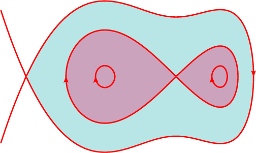
In the phase portrait 7.8 there is
also a third homoclinic orbit, which starts from the unstable
equilibrium point
, passing the two stable equilibrium
points
and
, and then going back to the point
. In that example, the homoclinic orbits are the boundaries
of the stability regions: the two darker regions in
figure 7.8 are the regions where the
system oscillates around the stable equilibrium points. In region with
a lighter color, the system oscillates around the two stable
equilibrium points.
Cycles always appear around stable equilibrium points and
homoclinic orbits always start and end at points of unstable
equilibrium. An equilibrium point where a homoclinic orbit exists is
necessarily an unstable equilibrium point because in one direction the
state of the system moves away from the point, but in another
direction the state approaches the point.
Note that in cycles the system passes repeatedly through
the same points in phase space, whereas in homoclinic
orbits the system never passes twice through the same
point in phase space.
The plot of the position
and velocity
versus time
(figures 7.9
and 7.10 ) can be obtained using the
option versus_t of the
program plotdf or with a menu
button.
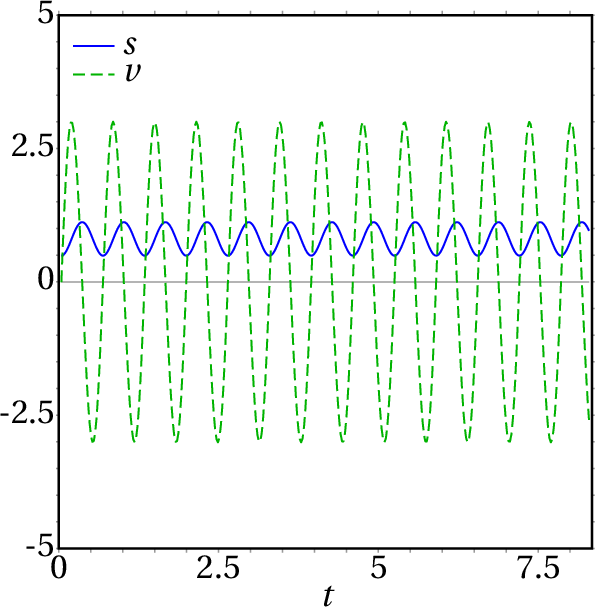
Figure 7.9: Position and velocity as a function of time in the
case of a cycle.
The plot of the state variables with respect to time in the case of
the cycle, shown in figure 7.9, shows
the periodic oscillation of the variables. The combination of these
two variables in phase space produces an ellipse around the point
(0.8102, 0) in the phase portrait 7.8.
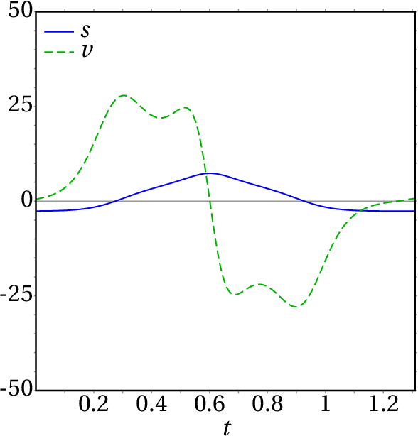
Figure 7.10 shows the non-periodic
oscillation of the state variables with respect to time for the
homoclinic orbit that approaches the equilibrium point (-2.652,0) in
the phase portrait 7.8.
Figure 7.10: Position and velocity as a function of time in the
case of a homoclinic orbit.
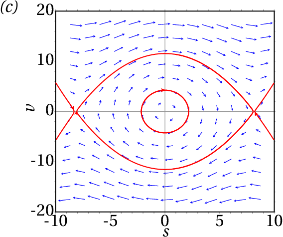
There are also heteroclinic orbits in some dynamical
systems. The phase portrait 7.11 shows
an example. In the triangle near the center of the portrait, the three
vertices are unstable equilibrium points. The three sides of the
triangle are three different evolution curves, which have no points in
common because the three vertices are not part of any of those 3
segments. Each segment starts from an equilibrium point and ends at
the next point, completing a cyclic sequence of points and curves,
with equal number of points and curves connecting them.
A heteroclinic orbit is formed by a sequence of
evolution
curves and
equilibrium points. The first curve starts at the first
point and ends at the second point, the second curve starts at the
second point and ends at the third point, and so on until the last
curve that ends at the first point.
Figure 7.11: Phase portrait with a heteroclinic orbit.
7.4. Conservative systems
In some dynamical systems it is possible to find a function
of the state variables which defines all the evolution curves in
phase space. Each possible evolution curve is defined by the
equation
(7.8)
With different values of the constant
. The function
is
called Hamiltonian
of the system and the systems in which it is possible to find such
function are called conservative
or Hamiltonian systems.
Since the state variables are functions of time
, any function
of the state variables is a function that depends only on
time. In the case of
equation 7.8 implies that
along any evolution curve; namely, the value of the function
remains constant as the system evolves. To compute the derivative
we use the chain rule for composite functions:
(7.9)
Substituting the evolution equations 7.2,
we obtain
(7.10)
One way to ensure that the result is null, for any values of the
state variables, is choosing a Hamiltonian that satisfies the
following conditions:
(7.11)
And it then follows that
(7.12)
We then conclude that any dynamical system
,
is conservative if, and only if,
its divergence is
zero:
(7.13)
When the dynamical system is equivalent to a second-order
differential equation
, the evolution
equations 7.6 make the previous condition
simpler:
(7.14)
Namely, the system is conservative if the function
does not
depend on
(that is equivalent to saying that the expression of the
second derivative
depends only on
and not on
).
In the case of mechanical systems, with evolution equations
obtained from Newton's law
, the necessary
and sufficient condition for the system to be conservative is that the
tangential force does not depend on the velocity
. In that case,
the Hamiltonian is defined by the following conditions:
(7.15)
Leading to the function,
(7.16)
which is the mechanical energy — kinetic plus potential
energies — per unit mass:
(7.17)
The two systems considered in
examples 7.1
and 7.3 are both conservative. In
example 7.3, the potential energy along
the trajectory is
And the Hamiltonian of the system is then
(7.18)
The evolution curves of the system are all the level curves of the
Hamiltonian
, on the phase plane
. Maxima's
program ploteq
can be used to plot level curves. Its syntax is similar to that
of plotdf, but the first
argument must be the expression of the Hamiltonian
, instead of the
list of components of the phase velocity:
Figure 7.12 shows the result, after
plotting some curves by clicking on some points.
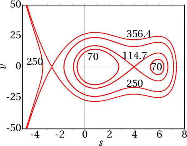
Figure 7.12: Level curves of the Hamiltonian of example
7.3.
The plot is similar to the plot already obtained
with plotdf in
figure 7.12. The main difference is the
absence of arrows indicating the direction of the time evolution of
the system, but since the horizontal component of the phase velocity
is the velocity itself, it is already known that all the curves above
the
axis move from left to right (
positive) and all the curves
below the
axis move from right to left (
negative).
It is important to understand that
figure 7.12 shows 9 possible different
motions, corresponding to 9 different evolution curves: 2 cycles, with
, each around one of the two stable equilibrium points. A cycle
with
, which goes around the two stable equilibrium points and
the unstable equilibrium point between them. Two homoclinic orbits,
both with
, Which begin and end at the unstable equilibrium
point and each one going around one of the stable equilibrium points;
114.7 is the value of
at the unstable equilibrium point, up to one
decimal digit. At the second unstable equilibrium point, the value
of
is 356.4 and there are three evolution curves with this value of
: a homoclinic orbit that goes around the other 3 equilibrium
points, a curve that starts at the unstable equilibrium point and
another one that ends at that point. On the left side of these last
two curves there are branches of hyperbolas that approximate
asymptotically these two curves, with values of
lower than
356.4. Figure shows one of them, with
.
As discussed in chapter 6 (work
and energy), the possible motions of a system whose resultant force is
conservative are easier to analyze in a plot of the potential
energy. In the case of example 7.3,
figure 7.13 shows the plot of the
potential energy per unit mass,
. The two stable equilibrium
points are marked with solid circles and the two unstable equilibrium
points with open circles.
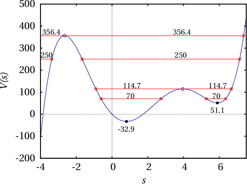
Figure 7.13: Potential energy per unit mass in
example 7.3 and 9 possible motions for
some values of
.
An important property is:
In a conservative mechanical system, the stable equilibrium
points are all local minima of the potential energy and the unstable
equilibrium points are all local maxima of the potential
energy.
The same 9 evolution curves that were plotted in the phase
portrait 7.12 are also shown in
figure 7.13. Each evolution curve
corresponds to a horizontal line segment, with a constant value of
, including only the points where
is bigger than
. Remember
that in this case
; namely, at each point in one of the
horizontal segments,
is equal to twice the vertical distance
from the point to the plot of
. For each value
there are two values of the velocity, with the same absolute value but
opposing signs, corresponding to the passage of the evolution curve
above and below the
axis in the phase portrait
(figure 7.12). At the points marked
with asterisks the velocity is zero, as in the equilibrium points, but
the tangential acceleration (slope of
times −1) is
not. Therefore, at those points the direction of motion of the system
is reversed.
The curves with
are motions in which the system can
start from
(less than the value of the unstable
equilibrium point), with
, passing through all 4 equilibrium
points and then stopping at
, where its direction of
motion is reversed, repeating the same motion but in the opposite
sense.
The two plots 7.13
and 7.12 show the same information in two
different ways. From one of these two plots one can figure out how the
other one will look like. In fact,
figure 7.12 was created by looking at
the values of
for each of the points marked with asterisks in
figure 7.13 and then entering those
values, followed by 0 (velocity), in the "Trajectory at" field of the
configuration menu of ploteq.
One can picture the plot of the potential energy per unit mass as a
gutter on a vertical plane, where a sphere is let to roll freely,
without loosing any energy by friction. Placing the sphere at a point
where the height of the gutter is a local maximum, it can remain at
rest but a small impulse causes it to roll down, moving away from that
maximum point (unstable equilibrium). If the sphere is released from
rest near a point where the height is a local minimum (stable
equilibrium), it rolls down to the minimum, speeding up, and the it
goes up on the opposite side, slowing down until it stops. If the
sphere does not lose any mechanical energy, the height of the point
where it stops is the same as in the point where it was
released. Thus, the sphere rolls down again and returns to the
starting point, repeating the cycle indefinitely.
Questions
(To check your answer, click on it.)
The resultant tangential force on a particle is
. At
The particle is at rest in
. Where will the particle be after a very long time?
Very far away, in
Moving around
In
In
Moving around
Which of the following is a necessary and sufficient condition for
a system to be autonomous?
It has no unstable equilibrium points.
It does not depend on any other systems.
It evolves spontaneously, without the need for external agents.
Its state does not depend on time.
Its evolution from an initial state is the in different instants.
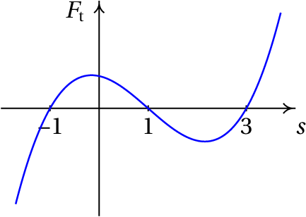
The figure shows the plot of the tangential component of the
resultant force
, acting on a body. Which of the
following statements is true of about the equilibrium points of the
body?
is stable and
unstable.
is stable and
unstable.
iIs stable and
unstable.
and
are both stable.
and
are both unstable.
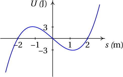
The figure shows the plot of the potential energy
along the
trajectory for a conservative mechanical system. At the initial time
the mechanical energy is 5 J, the position
and the velocity is
in the positive sense of
. How will the system move?
It oscillates around
It oscillates around
It moves to
and then returns, remaining at rest in
It remains at rest in
It moves to
and then in the negative direction, towards
.
What is the phase velocity of the conservative system with
potential energy along the trajectory
and mass
?
Problems
A 0.150 kg ball is thrown vertically upward from
(the
axis
points up vertically). Neglecting the air resistance, the mechanical
energy remains constant.
(a) Plot the phase portrait for
, showing 4 different
evolution curves (use the value 9.8 m/s2 for
). For each
curve, explain the meaning of the points at which the curve intersects
the two axes.
(b) In the phase portrait shown in the previous item, plot the
evolution curve of a ball that after falling freely to the ground
bounces back being thrown up vertically with the same speed it hits
the ground.
Explain which of the problems in chapter
1 describe autonomous, non-autonomous, conservative or
non-conservative systems. Plot the phase portrait of the system in
problem 6, showing the
evolution curve for the initial conditions given.
Consider the 3 cases in
problem 8
of chapter 1:
(SI units) (a)
, (b)
, (c)
. In each case find the equilibrium points, determine what
kind of points they are, plot the phase portrait and determine whether
there are cycles, homoclinic orbits or heteroclinic orbits.
A particle with mass 1 kg moves along the
axis. In SI units, the
tangential force on the particle is given by the expression
.
(a) Determine the equilibrium points of the system.
(b) Find the expressions for the potential and mechanical energies
in terms of
and the velocity
.
(c) Write down the evolution equations and say what kind
of dynamical system they represent.
(d) Classify each of the equilibrium points.
(e) Determine whether the system has cycles, homoclinic
orbits or heteroclinic orbits, and if so, represent one of those curves
in the phase portrait.
A particle with mass 1 kg moves along the
axis, under the effect of a single conservative force
with potential energy given by the expression (SI units)
(a) Determine the expression for the force as a function of
.
(b) Find the equilibrium points of the particle in phase
space (
,
), where
is the velocity.
(c) Classify each of the equilibrium points.
(d) Determine whether the system has cycles, homoclinic
orbits or heteroclinic orbits, and if so, represent one
of those curves in the phase portrait.
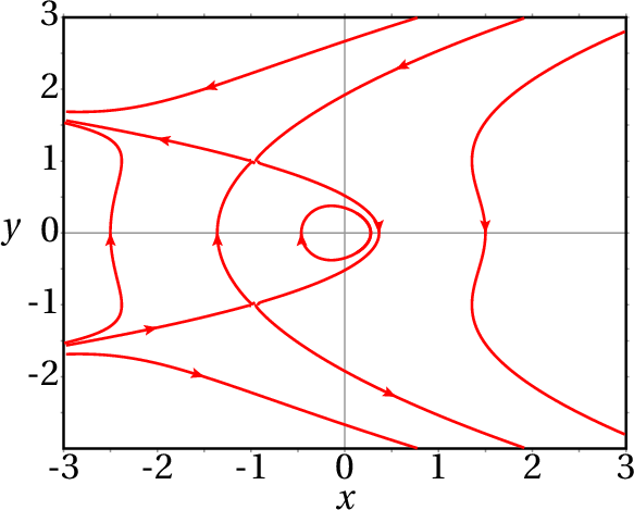
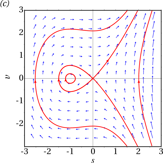
The figure shows the phase portrait of the dynamical system with evolution
equations:
(a) Determine whether the system has any cycle, homoclinic
orbit or heteroclinic orbit.
(b) Explain why the following statement is wrong:
"The phase portrait includes two parabolic evolution curves that
intersect at two points."
The total tangential force on a body with mass equal to 1 kg is
.
(a) Find the equilibrium points and determine whether
they are stable or unstable.
(b) Determine the potential energy along the path as a
function of
, assuming
at
, and compute
the potential energy at each equilibrium point.
(c) Represent the phase portrait of the system, showing
the 4 evolution curves corresponding to the following
values of the mechanical energy: 0, a value smaller
than the energies at the equilibrium points, a value
between the energies of the two equilibrium points and
a value greater than the energies at the equilibrium
points.
(d) Compute the position
where the body can be at
rest without being in equilibrium, with total energy
equal to zero. Explain how would be the motion of the
body starting from that initial state.
A particle with mass
moves under the action of a resultant force with
tangential component:
where
and
are two positive constants.
(a) Find the equilibrium points and show that they are
all stable.
(b) Explain the possible motions of the particle.
(c) Plot the phase portrait with a system of units where
,
and
are all equal to 1.
The equation of motion of a
simple pendulum is
(problem 6
of chapter 6)
The state variables are the angle with the vertical,
, and the derivative of this angle,
.
(a) Write down the evolution equations of the system.
(b) Find a Hamiltonian
by solving
Hamilton' equations:
(c) Analyzing the plot of the potential energy
(Hamiltonian with
= 0), show that the system
has many heteroclinic orbits and cycles but no
homoclinic orbit.
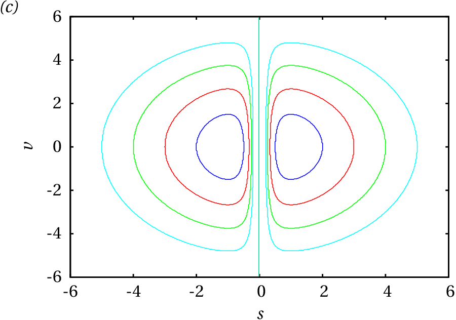
The mechanical energy of a particle with
mass
moving along the
axis remains constant and
its potential energy is:
where
and
are two positive constants.
(a) Determine the force acting on the particle.
(b) Find the equilibrium points and say whether they are
stable or unstable.
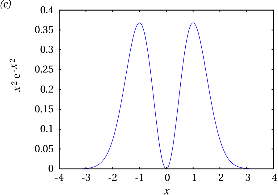
(c) Plot the potential energy for
and
.
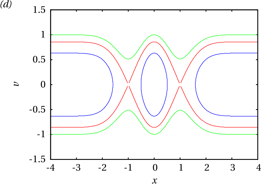
(d) Plot the phase portrait for
, showing the
heteroclinic orbit and one of the cycles.
Answers
Questions: 1. B. 2. E. 3. B. 4. E. 5. A.
Problems
The two symmetrical points where each parabola
intersects the axis of the velocity represent the
state when the particle is thrown from the ground and
when it falls back to the ground. The vertex of each
parabola, on the position axis, is the state at the
point where the ball reaches its maximum height.
(b) The ball follows one of the parabolic curves in
phase space, and when it reaches the point on the
negative side of the velocity axis, it passes instantly
to a point on the positive side of the velocity axis,
where it links to another parabola.
Autonomous and conservative systems in problems 3, 6, 7, 8,
and 9. Autonomous but non-conservative systems in problem 10.
Non-autonomous and therefore non-conservative systems in problems 2, 4, 5
and 11. The phase portrait for problem 6 is the following:
When
or
There is only one stable
equilibrium point, in
,
; all evolution curves
are cycles and there are no orbits. When
there
are two unstable equilibrium points
and
(
) and a stable equilibrium point
,
; there is a heteroclinic orbit and all the evolution
curves within it are cycles; there are no homoclinic
orbits.
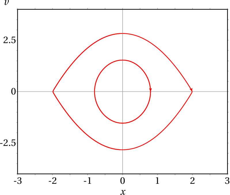
(a) (
,
) = (0, 0), (2, 0) and (−2,
0). (b)
(c)
,
.
It is an autonomous and conservative dynamical system.
(d) (−2, 0) is unstable, (0, 0) is stable and
(2, 0) is unstable. (e) There are infinite cycles,
a heteroclinic orbit and no homoclinic orbits. The following
plot shows one cycle and the heteroclinic orbit:
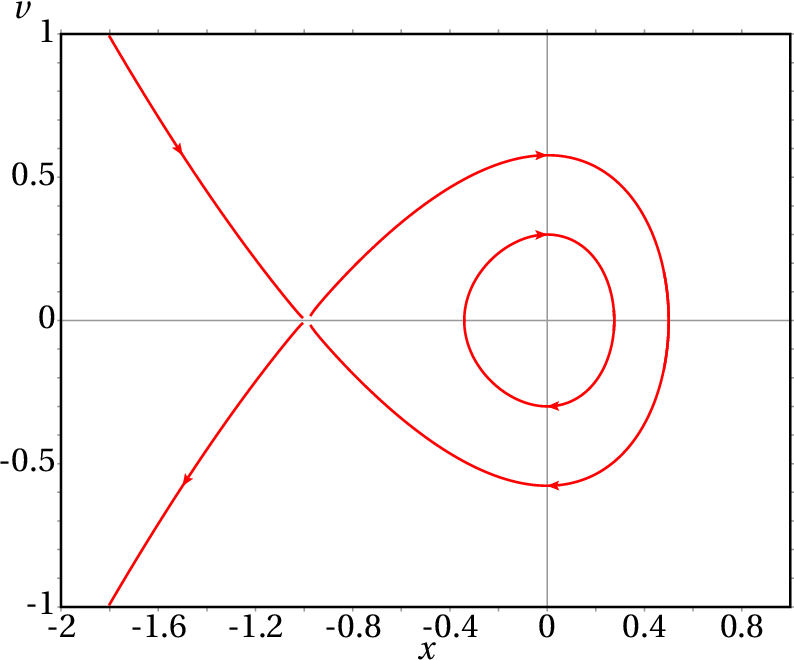
(a)
(b) (0, 0) and (−1, 0)
(c) (0, 0) is stable and (−1, 0) is unstable.
(d) There are infinite cycles, a single homoclinic
orbit, and no heteroclinic orbits. The following plot
shows one cycle, the homoclinic orbit, and the other two
evolution curves approaching the unstable equilibrium
point:
(a) There is a heteroclinic orbit between the
unstable equilibrium points (−1, 1) and (−1,
−1) and no homoclinic orbits. All the evolution curves
in the region bounded by the heteroclinic orbit are
cycles. (b) The two parabolas are actually 6
different evolution curves which approach asymptotically
or move away from the two unstable equilibrium points,
without touching them. Evolution curves can never cross.
(a) A stable equilibrium point in
and an
unstable equilibrium point in
. (b)
. At the stable equilibrium point
J and at the unstable equilibrium point
.
(d)
; the body accelerates in the positive
direction of
, begins to slow down in
and approaches a state of rest in
.
(a) There are two equilibrium points:
. At both points the potential energy is
a local minimum and therefore the equilibrium is
stable. (b) The motion is always oscillatory, with
values of
always positive or negative, depending on
the initial state.
(a)
(b)
is the mechanical energy
divided
by the moment of inertia
:
(c) There are stable equilibrium points
equal to 0,
,
, … and unstable equilibrium points
in
,
, … Any value of
between
and
corresponds to a cycle. When
there is a heteroclinic
orbit that goes through all the unstable equilibrium points
,
, … There are no homoclinic orbits because any
straight line segment
Starts and ends at unstable equilibrium
points and does not intersect the curve
.
(a)
(b) A stable equilibrium point in
and an
unstable equilibrium point in
.
Wrong
Hint: Assume that the mass is 1, so the tangential
acceleration is equal to the tangential force, plot the
direction field and plot the curve of evolution that passes
through the point
,
.
(click to continue)
Correct
is a center and
a saddle point. The particle does
not have enough energy to go beyond the saddle point, so it
remains oscillating around the center.
(click to continue)
Wrong
Hint: Assume that the mass is 1, so the tangential
acceleration is equal to the tangential force, plot the
direction field and plot the curve of evolution that passes
through the point
,
.
(click to continue)
Wrong
Hint: Assume that the mass is 1, so the tangential
acceleration is equal to the tangential force, plot the
direction field and plot the curve of evolution that passes
through the point
,
.
(click to continue)
Wrong
Hint: Assume that the mass is 1, so the tangential
acceleration is equal to the tangential force, plot the
direction field and plot the curve of evolution that passes
through the point
,
.
(click to continue)
Wrong
An autonomous can have either stable or unstable
equilibrium points.
(click to continue)
Wrong
The acceleration does not necessarily have to be zero in an
autonomous system; therefore, there can be external forces,
exerted by external systems.
(click to continue)
Wrong
An autonomous system can have acceleration which is then
produced by the forces exerted by external agents. The way
the system evolves is then due to external agents.
(click to continue)
Wrong
The very existence of evolution curves implies that the
state does depend on time.
(click to continue)
Correct
Since the phase velocity does not depend on time, if the
system starts from a given initial state, its evolution will
always be the same, regardless of the value of the time when
the evolution started.
(click to continue)
Wrong
is unstable, because the force points to the left on
the left of that point and to the right on the right of the
point. Therefore, the system moves away from
.
(click to continue)
Correct
(click to continue)
Wrong
is unstable, because the force points to the left on
the left of that point and to the right on the right of the
point. Therefore, the system moves away from
.
(click to continue)
Wrong
is unstable, because the force points to the left on
the left of that point and to the right on the right of the
point. Therefore, the system moves away from
.
(click to continue)
Wrong
is stable, because the force points to the right on
the left of that point and to the left on the right of the
point. Therefore, the system moves towards
.
(click to continue)
Wrong
The system does not oscillate because it has enough energy
(5 J) to go beyond the local maximum of the potential energy
(3 J).
(click to continue)
Wrong
The system does not oscillate because it has enough energy
(5 J) to go beyond the local maximum of the potential energy
(3 J).
(click to continue)
Wrong
In order to remain at rest in
, the energy should
have the same value of the potential energy in that point (3
J).
(click to continue)
Wrong
In order to remain at rest in
, the energy should have
the same value of the potential energy in that point
(−3 J).
(click to continue)
Correct
the system moves until a turning point and reverses its
motion to the negative direction; since its energy (5 J) is
greater than the potential energy in all the points to the
left of the turning point, it will never stop again.
(click to continue)
Correct
The components of the phase velocity are the velocity
and the tangential acceleration
, which is
equal to the tangential force divided by the mass. The
tangential force is obtained differentiating
with
respect to
and multiplying by −1.
(click to continue)
Wrong
The components of the phase velocity are the velocity
and the tangential acceleration
, which is
equal to the tangential force divided by the mass. The
tangential force is obtained differentiating
with
respect to
and multiplying by −1.
(click to continue)
Wrong
The components of the phase velocity are the velocity
and the tangential acceleration
, which is
equal to the tangential force divided by the mass. The
tangential force is obtained differentiating
with
respect to
and multiplying by −1.
(click to continue)
Wrong
The components of the phase velocity are the velocity
and the tangential acceleration
, which is
equal to the tangential force divided by the mass. The
tangential force is obtained differentiating
with
respect to
and multiplying by −1.
(click to continue)
Wrong
The components of the phase velocity are the velocity
and the tangential acceleration
, which is
equal to the tangential force divided by the mass. The
tangential force is obtained differentiating
with
respect to
and multiplying by −1.
Hint: Assume that the mass is 1, so the tangential acceleration is equal to the tangential force, plot the direction field and plot the curve of evolution that passes through the point , .
(click to continue)