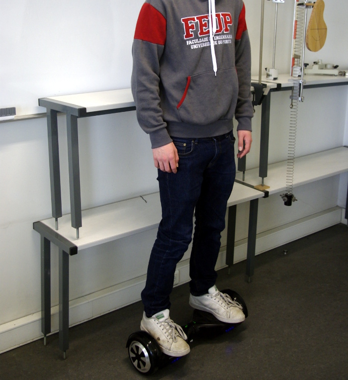
A hoverboard has just one axle with two wheels. The person
riding it can rotate around that axle as in a pendulum. A pendulum has
two equilibrium positions, one where its center of gravity is directly
below its axis, and in the other its center of gravity is directly
above the axis. The person riding the hoverboard is in that second
equilibrium position, which is unstable; if the center of gravity
moves slightly out of the vertical that passes through the axle, the
weight will make the rider move even further away from that vertical,
falling frontwards or backwards. The hoveboard has an automatic
control system that makes it move forward or backward, thus bringing
the center of gravity back to the equilibrium position. A pendulum
like that, oscillating around the stable equilibrium position by means
of an external force, is called an inverted pendulum. Other examples
of inverted pendulums are a Segway and a mono-cycle.
10.1. Linear approximation
Let us consider a continuous dynamical systems with two state
variables:
(10.1)
each of the functions
and
can be expanded as a
Taylor series, in the neighborhood of a point (
,
) in
phase space:
(10.2)
where the index
can be 1 or 2. If the point (
,
) is an
equilibrium point, then
and, therefore, the
first term of the two series is null. Changing the origin of
coordinates to the equilibrium point (
,
), that is, in a new
coordinate system:
,
, the first two terms in the
series expansion of the functions are,
(10.3)
Which is a linear combination of the new variables
and
, where
the constants multiplying the two variables are the values of the
partial derivatives at the equilibrium point (
,
). Substituting
these approximations into the system 10.1, we
obtain a linear system (
e
,
because
and
are constants).
(10.4)
this linear approximation is valid only in a neighborhood of the
origin (
,
), namely, for
and
near the
equilibrium point (
,
).
The square matrix in
equation 10.4 is
called Jacobian
matrix, represented here by
. Substituting the coordinates (
,
) of the equilibrium
point in the Jacobian matrix gives a constant matrix. At each
equilibrium point, a different matrix is obtained which defines a
linear system that approximates the nonlinear system in a neighborhood of the
equilibrium point. The eigenvalues and eigenvectors of each of these
matrices can be used to analyze the stability of the system near each
equilibrium point, in the same way that it is done for linear systems.
Example 10.1
Classify the equilibrium points and plot the phase portrait of the
system:
Resolution. It has already been shown in the
example 7.2
of Chapter 7 that this system has
four equilibrium points. Let us save the functions
and
and
the equilibrium points in two Maxima lists:
It is also convenient to define another list with the names of the
state variables:
(%i3)v: [x1, x2]$
The jacobian matrix, with two rows and two columns, is obtained using
Maxima's command jacobian, which requires two lists, with the
functions and the variables names.
(%i4)J: jacobian (f,v);
(%o4)
Substituting the coordinates of each equilibrium point, we obtain
the matrices of the linear systems that approximate the nonlinear
system in the vicinity of its equilibrium points. For example, at the
first equilibrium point,
(%i5)subst (equilibrio[1], J);
(%o5)
In order to study the stability of the system in the vicinity of
this equilibrium point, let us compute the eigenvalues of this
matrix.
(%i6)eigenvectors (%)$ (%i7)float (%);
(%o7)
The result shows 4 lists; the first list are the
eigenvalues, the second list are their multiplicities and
the last two lists are the eigenvectors corresponding to the
two eigenvectors.
At this equilibrium point, the eigenvalues are real, with opposite
signs; we then conclude that it is a saddle point. The fourth
equilibrium point is also saddle point:
Since the eigenvalues are complex, with the negative real part, the
equilibrium point is an attractive (stable) focus. Similar
calculations for the third equilibrium point show that it is also a
focus, but repulsive (unstable), because the real part of the
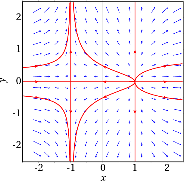
eigenvalues is positive. The phase portrait is created using the
command:
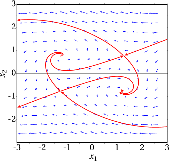
(%i14)plotdf (f, v, [x1,-3,3], [x2,-3,3])$
Figure 10.1 shows the
result. There is a single stable equilibrium point, an
attractive focus, at (
,
) = (1,265,
−0.7746). The other 3 equilibrium points are unstable:
two saddle points and a repulsive focus. The two evolution
curves shown near the repulsive focus at (
,
) =
(−1.265, 0.7746) and their continuation until the
saddle points delimit the stability region. When the initial
state of the system is in that region, the final state will
approach the stable equilibrium point.
Figure 10.1: Phase portrait of the system
,
.
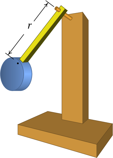
10.2. The pendulum
Figure 10.2: Pendulum.
The kind of pendulum that
we will study in this section consists of an object connected to a
rigid bar crossed by a fixed horizontal axis
(Figure 10.2). This type of pendulum can
rotate in a vertical plane making complete turns. The system has a
single degree of freedom,
, which is the angle that the bar
makes with the vertical. Let us set
when the pendulum is
in the lowest position and
in its highest position. The
angular velocity is
and the speed of the center of mass
is
where
is the distance from the center of mass
to the axis.
The kinetic energy of the pendulum is:
(10.5)
Where
is the total mass and
is the moment of
inertia with respect to the center of mass. According to the parallel
axes theorem 5.23,
is the moment of inertia
with respect
to the axis of the pendulum, which can be written as
, where
is the radius of gyration
relative to the axis. Therefore, the kinetic energy can be written
as
(10.6)
The gravitational potential energy is (setting zero energy at
)
(10.7)
Ignoring the air resistance, the Lagrange equation leads to
the equation of motion:
(10.8)
where
defines the effective length of
the pendulum. In the particular case of a
simple pendulum, in which the mass of the bar is negligible and the
disk is very small,
equals the distance from the center
of the dist to the axis (see
example 8.5
in Chapter 8 ).
The evolution equations are obtained by writing the derivative of
as the angular velocity
and the angular acceleration
as the derivative of the angular velocity:
(10.9)
These nonlinear equations can only be solved approximately using
some numerical approximation. The Maxima
program rk can be
used to obtain the numerical solution by the fourth-order
Runge-Kutta method. That program requires 4 input
parameters: a list with the expressions for the components
of the phase velocity, a list with the names of the state
variables, a list with initial values for those variables
and a range of values for the independent variable,
including the name of the variable, its initial value, its
final value and the length of the steps to be taken from the
initial to the final value. The output
of rk is a list of points
that approximate the solution; each point will have the
coordinates of the independent variable, followed by the
values of the state variables at that point.
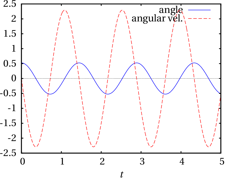
For example, for a pendulum with effective length
of 50 cm,
released from rest at an initial angle of 30°, the
approximate solution is obtained with the following command
(
and
stand for
and
):
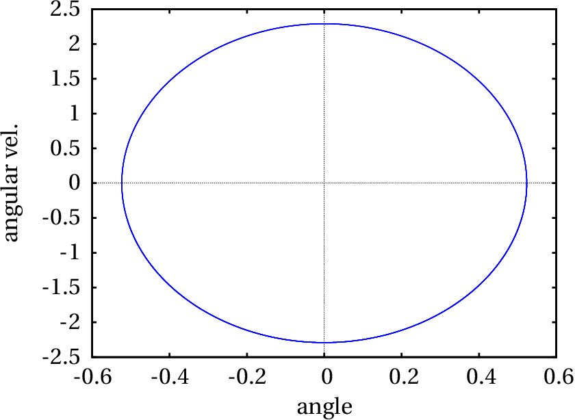
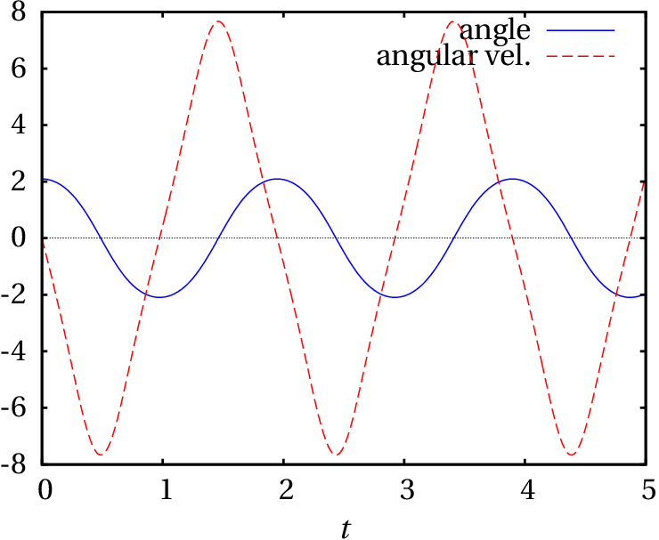
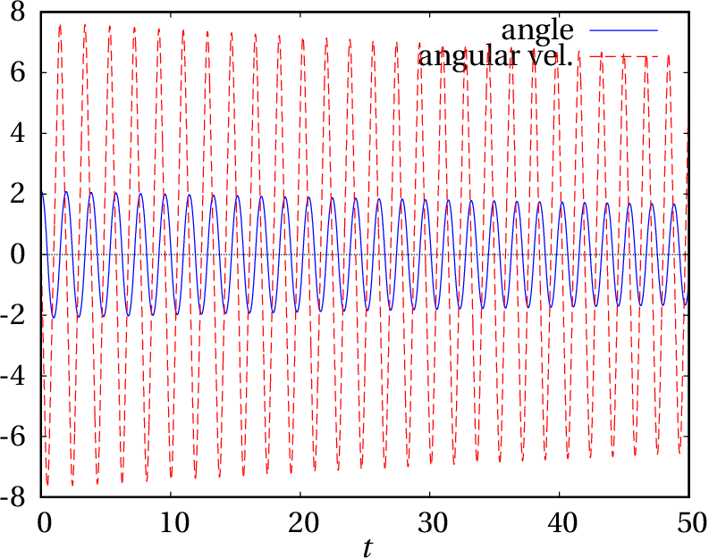
Figure 10.3: Oscillations of a 50 cm
pendulum with amplitude of 30°.
Looking at the list of values obtained for
, one
can conclude that the period of oscillation is between 1.44
and 1.45 s. The plots in
Figure 10.3 are very similar to
the plots for a simple harmonic oscillator. If the initial
angle is bigger, this similarity begins to disappear. For
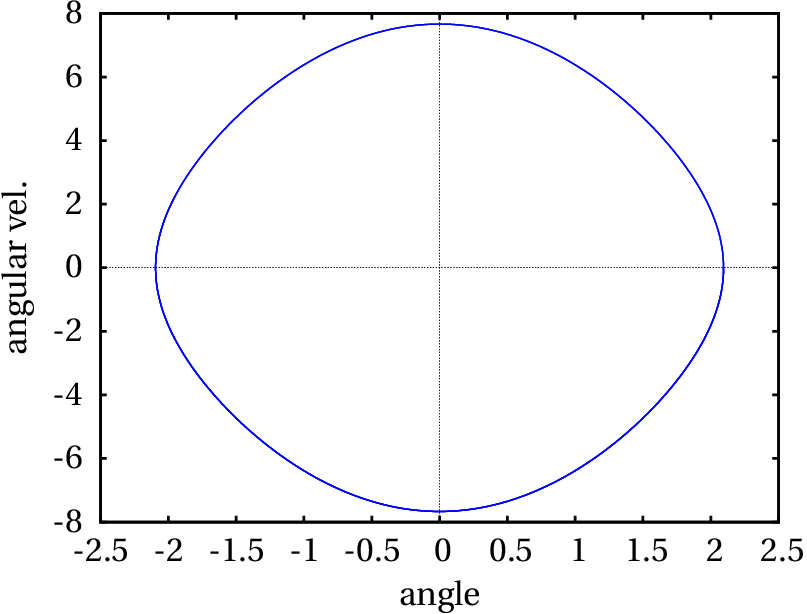
example, Figure 10.4 shows the
results obtained with an initial angle of 120°.
Figure 10.4: Oscillations of a 50 cm
pendulum with amplitude of 120°.
In this case the period of oscillation is between 1.94 and
1.95 s, which is bigger than in the case of 30°
amplitude.
In the two cases shown in
Figures 10.3
and 10.4, the evolution curve is a
cycle, which implies the existence of a stable equilibrium point
inside the cycle.
The equilibrium points of the pendulum, where the right
sides of equations 10.9 are
zero, occur at
,
,
…
and
.
The points at
,
,
… are
actually the same physical point, corresponding to the pendulum
passing through its lowest position after making some complete
turns. The points at
,
… are also
the same physical point, at the highest position of the pendulum.
10.3. Linear approximation of the pendulum
The Jacobian matrix obtained from the
equations 10.9 of the pendulum
is
(10.10)
At the equilibrium point in
(in general, 0,
,
,…), the matrix is:
(10.11)
which is the matrix of a simple harmonic oscillator,
discussed in
Example 9.4
of Chapter 9. Its two
eigenvalues are
, so the
equilibrium point at
is a center and if
the initial state of the system is close to that point, the
pendulum oscillates with angular frequency
. In the case of the 50 cm pendulum considered in
the previous section, this expression leads to a period of
1.42 s. Remember that this value is only an approximation,
which becomes better the smaller the amplitude; the period values
obtained in the previous from a numerical solution of the equations
section are more accurate.
In the neighborhood of the equilibrium point at
(in general,
,
,…), the
Jacobian becomes
(10.12)
which is the matrix of an inverted oscillator, discussed in
Example 9.3
of Chapter 9. The two
eigenvalues are
and the equilibrium point
is a saddle point (unstable equilibrium).
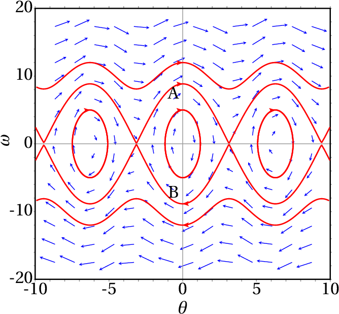
The phase portrait in the domain
will
show 3 centers (
, 0 and
) and 4 saddle points
(
,
,
and
). For the
cm
pendulum we can plot the phase portrait with the
command:
Figure :10.5 shows the
result. The angle
is in the horizontal axis and the
angular velocity
is in the vertical axis. The two
curves identified with the letters A and B form part of a
heteroclinic
orbit.
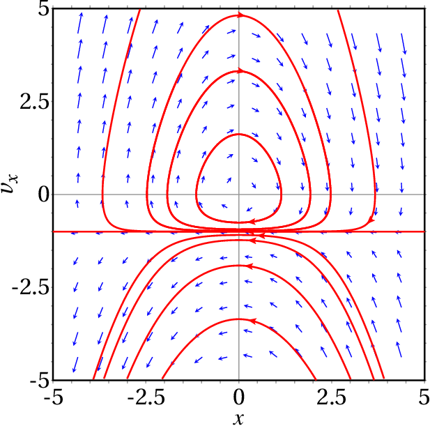
Figure 10.5: Phase portrait of a 50 cm
pendulum.
The heteroclinic orbits of the pendulum correspond to the
case when the mechanical energy of the pendulum is exactly
equal to the gravitational potential energy at the point of
maximum height. Since we are using as reference
, at the position
where the pendulum bar is horizontal (
), the
potential energy at the highest point is
. Each
of the curves A and B represent the motion starting with the
pendulum nearly at rest and very near its highest position,
descending and completing a full turn back to the highest
position, without further oscillation. The difference
between the heteroclinic orbits and cycles is that in
cycles the oscillations repeat indefinitely, whereas in a
heteroclinic orbit there is a single oscillation.
All the evolution curves in the region of phase space
inside the heteroclinic orbit are cycles. Those which are
closer to the heteroclinic orbit correspond to oscillations
in which the pendulum almost reaches its highest point, it
seems to stop there for a few moments and then moves down
again to the lowest point, repeating the same motion on the
other side of the vertical.
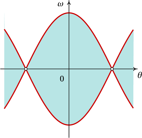
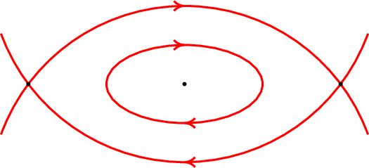
The heteroclinic orbits are also separatrices,
because they separate the phase space into a region where the pendulum
oscillates —the region shaded in
figure 10.6— and a region where the
pendulum keeps rotating in the same direction.
Figure 10.6: The heteroclinic orbits
delimit the regions where the pendulum
oscillates.
Figures 10.3
and 10.4 show that with a 30°
amplitude the linear approximation is quite good, since the
evolution curve is very similar to that of the simple
harmonic oscillator and the period is close to the period
obtained with the linear approximation, but with amplitude
of 120°, the linear approximation is no longer
accurate.
10.4. Multi-dimensional phase spaces
In autonomous mechanical systems, for each degree of
freedom there is an equation of motion, which implies two
state variables. Thus, the dimension of the phase space is
twice the number of degrees of freedom. If a system is not
autonomous the phase space has one more dimension, as shown
in the following section. Thus, the number of dimensions of
the phase space for a mechanical systems can be 2, 3, 4, 5,
…
In cases when the phase space has more than two dimensions
the plotdf program can not be used
to show the phase portrait. It is necessary to solve the
evolution equations for some specific initial values which
can then be used to plot some of the state variables.
10.4.1. Systems of non-autonomous equations
The general form of a system with
non-autonomous
differential equations is:
Each possible state of the system is characterized by the
values of the
variables
and time
; therefore,
each state is a point with
coordinates (
,
,…,
,
) and the phase space has
dimensions. The components of the phase velocity are the
derivatives of the coordinates of the state: (
,
,…,
,
). The expressions
for the first
components are given by the system of
differential equations and the last component
is always equal to 1 (derivative of
with
respect to
). Hence, a non-autonomous system with
equations is a dynamical system with
state
variables.
Such systems of equations can also be solved with
the rk program, without having
to include
among the state variables, nor the last
component of the phase velocity,
; the initial
value of
is given to rk in
the integration interval and not in the list of initial
values for the state variables. However, it must be
remembered that
is also a state variable in the cases
when the phase velocity depends on it.
Example 10.2
The differential equation:
is called Bessel. equation. Write the equation as a dynamic
system and identify its phase space.
Resolution. We regard
as another variable
:
(10.13)
so the second derivative
is equal to the first
derivative of
and the Bessel equation becomes:
solving for
we get,
(10.14)
Since this is not an autonomous equation, we consider the independent
variable
as another state variable, with the trivial evolution
equation:
(10.15)
The phase space has three dimensions (
,
,
). The corresponding
dynamical system is defined by 3 equations 10.13,
10.14 and 10.15.
10.4.2. Projectile motion
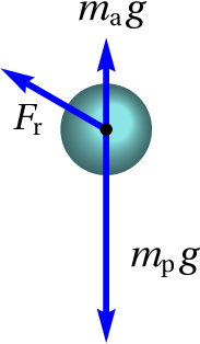
Figure 10.7: Projectile in the air.
As a projectile moves through the air, three external forces act on
it: its weight,
, the air resistance,
and the upward buoyant force
, where
is the mass of the projectile and
the mass of air
displaced by the projectile. This problem is similar to the free fall
studied in section
4.3.3 of chapter 4 , but the
resistance of the air is no longer vertical (see
figure 10.7). The weight and the buoyant force
are vertical, in opposite directions, and can be combined into a
single vertical force (effective weight) with magnitude
.
In the case of projectiles with density much larger than the
density of the air, the effective weight is very close to the weight
of the projectile
. In any case, the mass of the
projectile is usually measured by measuring its effective weight in
the air, so the measured value (
) of the projectile mass is really
and the effective weight is
.
The force of resistance of the air, being opposite to the velocity
of the projectile, points in different directions at different points
of the trajectory. As was explained in Chapter 4, in the case of air
the Reynolds number is usually high and we can assume that the air
resistance is proportional to the square of the velocity. If the
projectile is a sphere of radius
, the magnitude of
is given by equation 4.14
and the expression of the force is:
(10.16)
where
is the air density and
is the
tangential vector pointing in the direction of the velocity
vector:
(10.17)
Choosing a system of axes in which gravity points in the negative
direction of the
axis and the initial velocity
with
which the projectile is launched is in the
plane, the weight and
the force of air resistance are always in the plane
and the
projectile's trajectory will be on that plane. Thus, the velocity
vector is
and the air
resistance force is:
(10.18)
The weight vector is
. Newton's second law
leads to the acceleration components:
(10.19)
These equations must be solved simultaneously because the two
components
and
appear in the two equations. We can find a
numerical approximation to the solution.
Let us compare obtain the trajectories of two different spheres,
launched with the same initial velocity, and compare them with the
parabolic trajectory they would have followed in vacuum, without air
resistance. Consider the case where the initial velocity is 12 m/s, at
an angle of 45° above the horizontal; the components of the initial
velocity are,
Starting with the easiest case, launching the projectile in vacuum,
the acceleration components are
and
. The state
of the projectile is (
,
,
,
) and the components of
the phase velocity are (
,
,
,
). The components of
the initial velocity have already been computed
in (%i19) and let us assume the projectile
is launched from the origin, so the initial values for
and
are
zero. To integrate the equations of motion from
to
s,
with time increments of 0.01 s, we use the command:
The 5 components of that point are time, position coordinates, and
velocity components. This result shows that at
the ball is
already falling, because
is negative, and it has already dropped
below the initial height, because
is also negative.
In order to obtain the trajectory until the ball returns to the
initial height
, it is necessary to extract only the points from
list tr1 with third positive component
(
). We can scan the entire list comparing the third element of each
point with 0 until we find the first point where that element is
negative. This can be achieved with Maxima's
command sublist_indices:
The command lambda was used to define an operator that compares the third element of the input given to it with zero. The sublist_indices command goes through the tr1 list, passing each element as input to that operator and when that operator produces the result "true", the index of current list element is appended to a sublist. The command first selects only the first element in that sublist, in this case the index of the first point where
is negative. As such, only the first 174 points on the list are of interest; since our goal is to plot the trajectory, we extract the coordinates
and
of the first 174 points into another list:
(%i23)r1: makelist ([tr1[i][2], tr1[i][3]], i, 1, 174)$
We will now repeat the same steps for a tennis ball and a
ping-pong ball, taking into account the resistance of the air. The
density of the air is approximately 1.2 kg/m3. It is
convenient to define a function that returns the constant that appears
in the equations of motion 10.19, for given
values of the radius and the mass of a ball; and we also define the
expression of the magnitude of the velocity so as not to have to write
it several times:
A typical tennis ball has a radius of approximately 3.25 cm and
mass 62 grams. In the command (%i20) it is
necessary to replace the acceleration of gravity by the two
acceleration components (equations 10.19)
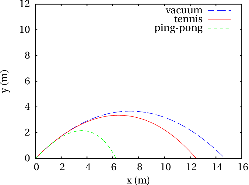
Figure 10.8: Trajectories of a ball in vacuum, a tennis ball in air and a ping-pong ball in air.
The trajectories of the balls in the air are not parabolas because
they curve more at the end, ending with a more vertical drop. The
effect of air resistance is more visible on the ping-pong ball;
although it is smaller than the tennis ball, the air resistance slows
it more, due to its lower density. Launched with the same velocity,
the horizontal ranges of the ping-pong and tennis balls are 6.2 m and
12.4 m. The hypothetical horizontal range of the two balls, if air
resistance could be eliminated, would be 14.7 m.
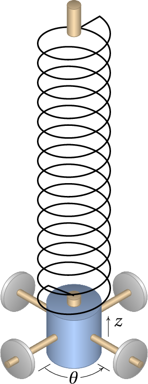
10.4.3. Wilberforce pendulum
Figura 10.9: Wilberforce
pendulum.
A Wilberforce
pendulum (Fig. 10.9) consists of a
cylinder that hangs from a very long vertical spring. When a spring is
stretched or compressed, each turn changes slightly in size; in
the Wilberforcependulum, the large number of turns in the spring
makes this change more visible; thus, as the spring oscillates up and
down, it also winds or unwinds leading to rotation of the cylinder
around its vertical axis.
This system has two degrees of freedom, the height
of the
center of mass of the cylinder and the angle of rotation of the
cylinder,
. If
and
are set in the equilibrium
position, it is possible to ignore the gravitational potential energy
that can be eliminated from the equations with a change of variables
(see problem 4
in Chapter 9). The elastic
potential energy has 3 terms, which depend on the elongation
of
the spring and its angle of rotation
. The kinetic and
potential energies are,
(10.20)
where
,
and
are elastic constants of the
spring. Lagrange equations, ignoring air resistance and other
dissipative forces, lead to the following equations of motion:
(10.21)
To solve the evolution equations numerically, it is necessary to
give some typical values for the mass, the moment of inertia and the
elastic constants,
(%i33)[m, I, k, a, b]: [0.5, 1e-4, 5, 1e-3, 0.5e-2]$
The solution in the time interval from 0 to 40, with initial
conditions
cm and the other variables equal to 0, is obtained
with the following command:
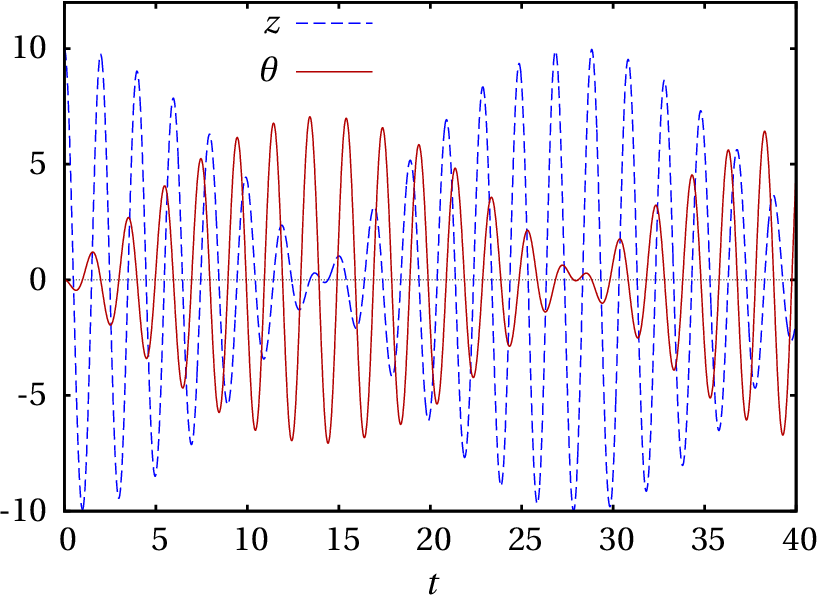
Figure 10.10 shows the plot obtained for
the angle
and the elongation
, multiplied by a factor of
100 so that it is visible on the same scale of the angle.
Figure 10.10: Elongation and angle of rotation in a
Wilberforce pendulum.
The graph shows an interesting feature of the Wilberforce pendulum:
if the pendulum is made to oscillate without rotating, the amplitude
of the linear oscillation decreases gradually, while the cylinder
begins to rotate with torsional oscillation that reaches a maximum
amplitude when the cylinder stops moving vertically. The amplitude of
the torsional oscillation then begins to diminish as the linear
oscillation grows again. This intermittence between vertical
displacement and rotation repeats itself indefinitely.
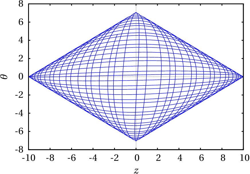
The projection of the phase portrait in the
and
plane
is shown in Figure 10.11.
Figure 10.11: Phase portrait on the plane formed by elongation and angle.
This system has two angular frequencies. The longitudinal angular
frequency and the torsion angular frequency,
(10.22)
The cylinder in a Wilberforce pendulum usually has four nuts that
can be displaced, increasing or decreasing the moment of inertia, to
make the two frequencies very similar and the alternating effect
between linear and rotational oscillations more visible. The values
that we used for the parameters were chosen to guarantee two equal
frequencies.
Questions
(To check your answer, click on it.)
The approximate value of the period of a pendulum with length
is
, where
is the acceleration of
gravity. This expression is a good approximation only in some
situations. If the angle
is zero at the stable equilibrium
point, which of the following conditions guarantees that this
expression is a good approximation of its real value?
angular
velocity small.
acceleration
of gravity small.
length
small.
maximum
value of
small.
air
resistance negligible.
If
represents the speed of a particle and
its position
along its trajectory, the expression of the total tangential force
on the particle is
. How many
equilibrium points does this system have?
1
2
3
4
0
Which of the following is the Jacobian matrix of the system with
evolution equations
,
?
The evolution equations of a dynamical system with phase space
(
,
), are
,
. Which of the
following vectors has the same direction as the phase velocity in
(1, 2)?
Regarding the phase portrait shown in the figure, what kind of
equilibrium point is (1, 0)?
attractive
knot
repulsive
focus
saddle point
attractive
focus
repulsive
knot
Problems
A particle of mass
, moves along the x-axis
under the action of a total force
which depends on the
position
and the velocity
. For each of the following cases
find the equilibrium points, say what kind of points they are
(stable or unstable, center, focus, knot or saddle) and plot the
phase portrait showing the most important curves:
(a)
(b)
In each of the following cases find the
equilibrium points and eigenvalues of the Jacobian matrix at those
points, and classify each of the equilibrium points:
(a)
(b)
(c)
(d)
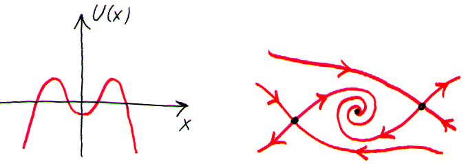
The following plot shows the phase portrait of a
system with only 3 points of equilibrium, in the idealized case
where there is no friction. Sketch by hand the plot of the potential
energy and the modified phase portrait when friction forces are
considered.
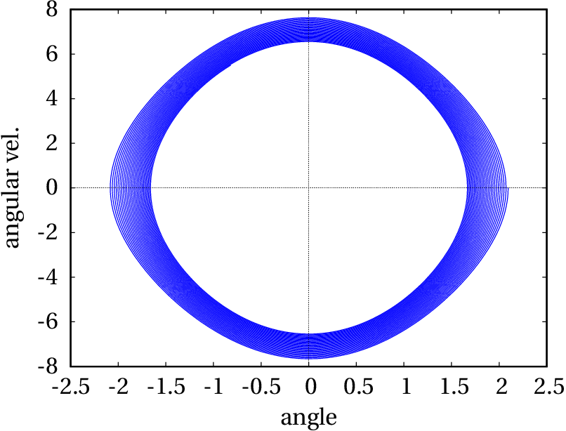
The angular amplitude of a swinging pendulum
decreases, due to air resistance and friction in the axis. Consider
a pendulum of length
cm and mass
kg, in which the
friction in the axis can be neglected but the air resistance
not. The equation of motion is
Equation 8.8
If most of the mass
is concentrated in a sphere of radius
cm, the expression for the constant
is given by
Equation 4.14:
, where
kg/m3 is
the density of the air. Plot the graphs of
,
;
plot the evolution curve in phase space and explain its physical meaning
in the following two cases:
(a) The pendulum is released from rest at an initial angle
.
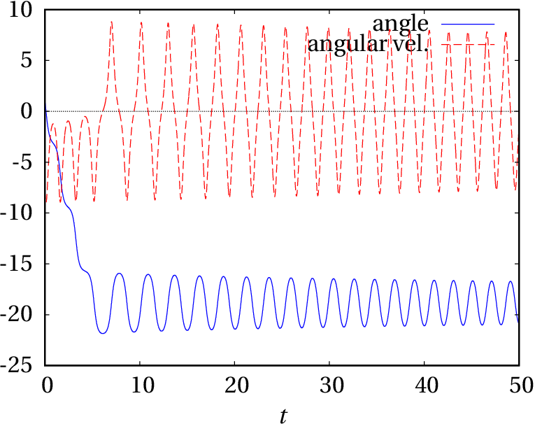
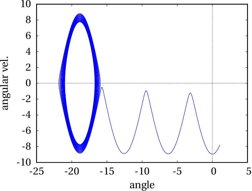
(b) The pendulum is released from
, with initial
angular velocity
s-1.
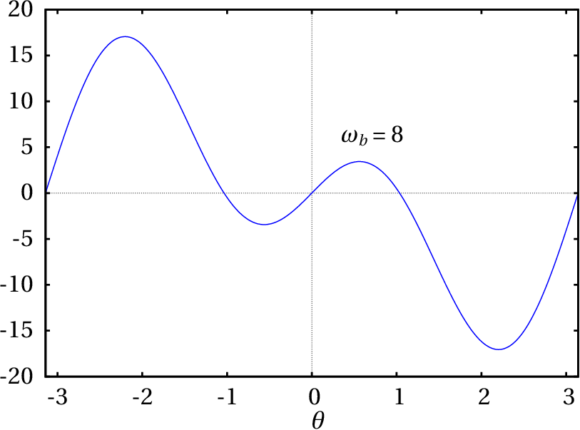
The base of the pendulum of
Figure 10.2 rotates in the horizontal plane,
with constant angular velocity
, while the pendulum
swings.
(a) Show that the equation of motion is:
where
is the distance from the center of mass to the axis and the
effective length
equals the square of the gyration radius, divided
by
.
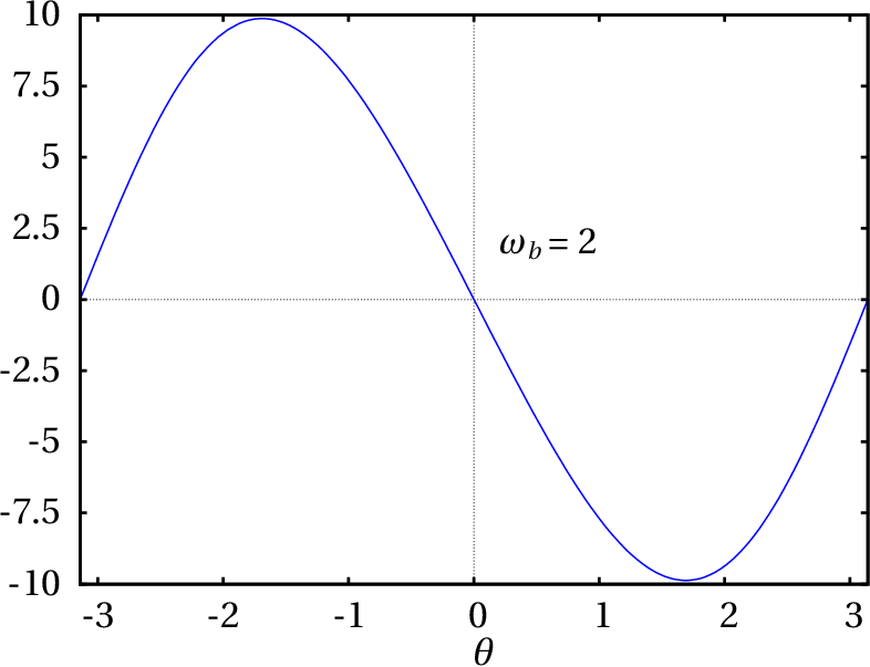
(b) Plot the graph of
as a function of
, between
and
, for a pendulum with
m and
s-1. Repeat the plot by changing the value of
to 8 s-1. Based on the two plots, find in each
case the position
of the stable and unstable equilibrium
points.
(c) Show that when
, there is a single
stable equilibrium point at
and a single unstable equilibrium
point at
.
(d) If
, show that the equilibrium
points at
and
are both unstable and two more
stable equilibrium points appear at
, where
is an angle between zero and
.
In the trajectory of the ping-pong ball obtained in
section 10.4.2 ,
the horizontal range of the ball is approximately the value of the
coordinate
of the last point in list r1. Repeat the
calculations changing the angle of the initial velocity above the
horizontal; use the values 35°, 36°, 37°, 38°, 39°, and 40°. Make a
table with the values of the horizontal range for each of those
angles. From that table, determine the angle that leads to the
biggest horizontal range. From the result of
Problem 12
in Chapter 6, show that in
vacuum the angle that produces the maximum range is 45°.
To analyze the nonlinear differential equation
,
(a) Write the evolution equations of the dynamical system
equivalent to the equation.
(b) Find the equilibrium points of the system.
(c) Find the Jacobian matrix.
(d) Classify each of the equilibrium points.
(e) If in
the values of
and its derivative are
and
, determine (numerically) the values of the variable
and its derivative at
.
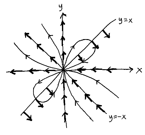
The dynamical system with evolution equations:
has a single equilibrium point at the origin. The Jacobian matrix at that
point is equal to zero and therefore the (null) eigenvalues can not be
used to classify that equilibrium point. Use the following method to
analyze the phase portrait of the system:
(a) Find the unit vector in the direction of the phase velocity at
points on the
axis and at points on the
axis.
(b) Find the unit vector in the direction of the phase velocity at
points on the two lines
and
.
(c) Sketch by hand the unit vectors found in the previous items at
several points on the 4 quadrants of phase space, and plot some evolution
curves following those phase velocity directions. On the basis of that
plot, what kind of equilibrium point you think the origin is?
(d) Draw conclusions about the existence of cycles, homoclinic
orbits or heteroclinic orbits and, if they exist, how many.
A particle of mass
moves on the
plane
under the action of a conservative force with potential energy,
where
and
are two positive constants. The trajectories
of the particle obtained with different values of these constants
are called Lissajous
figures.
(a) Find the two equations of motion for
and
.
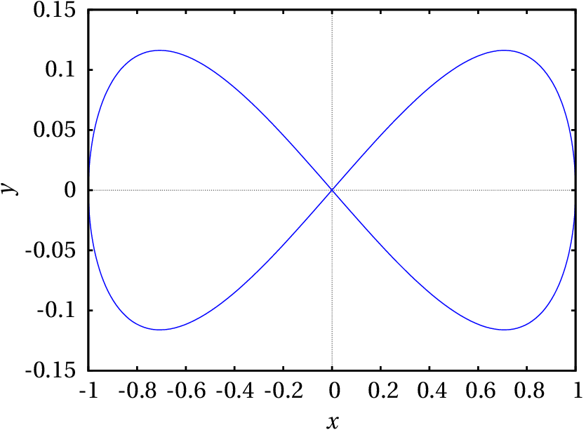
(b) Solve numerically the equations of motion, in the case
,
and
(SI units), between
and
,
if the particle starts from point (1, 0) with initial velocity
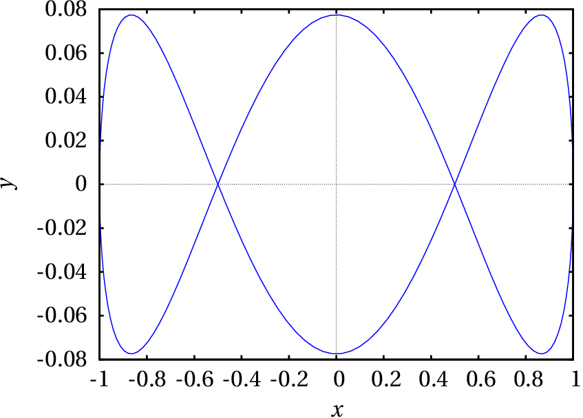
. Plot its trajectory on the
plane.
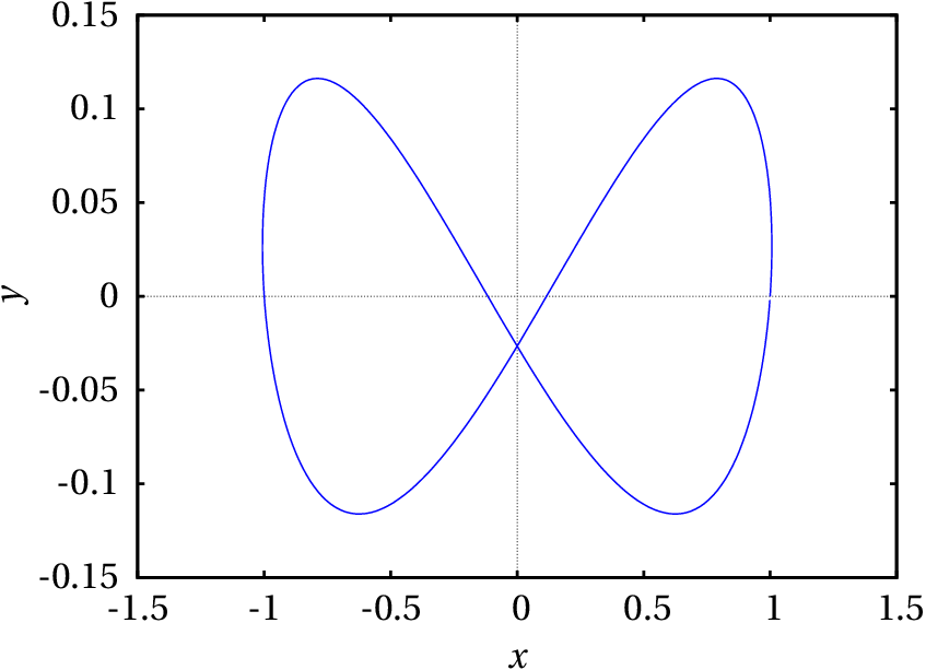
(c) Repeat the previous item, but now with the particle
starting from (1, 0) with initial velocity
.
(d) Note that the system can be considered as a set of two
independent harmonic oscillators, in the directions
and
. Compute the oscillation period for each of those two
oscillators and find the ratio between them.
(e) Repeat the procedure in item c, changing the value
of
to 18. What relationship do you see among the trajectories
and the ratio
?
Any celestial body (planet, comet, asteroid,
space probe, etc.) of mass
in the solar system has a
gravitational potential energy produced by the Sun, which is
responsible for the elliptical orbits of these bodies. The
expression for the potential energy is
where
is the universal gravitational constant,
is the mass
of the Sun and the coordinates
and
are measured on the plane
of the orbit of the celestial body, with the Sun qt the origin. If
distances are measured in astronomical units, AU, and the time in
years, the product
will be equal to
.
(a) Find the equations of motion of the celestial body in
units of years for time and AU for distances.
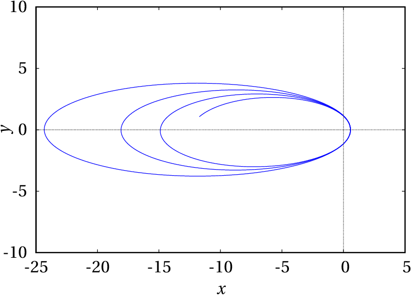
(b) Comet Halley reaches a minimum distance from the Sun
equal to 0.587 AU. At this point, its velocity is maximal, equal to
11.50 AU/year, and perpendicular to the segment from it to the
Sun. Find numerically the orbit of Halley's comet, from the
initial position
, with initial velocity
, using time intervals
years. Plot the orbit from
to
years. What can you
conclude about the numerical error?
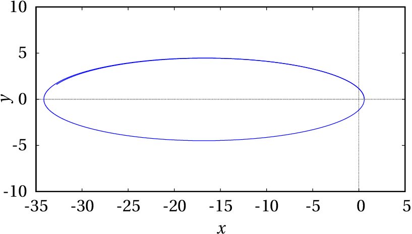
(c) Repeat the procedure of the previous item with
years and plot the orbit from
to
years. What can you conclude about the numerical error?
(d) Find the maximum distance that the Halley comet moves
away from the Sun, and compare the comet's orbit with the
orbits of the farthest planet, Neptune (orbit between 29.77 AU and
30.44 AU), and the closest planet to the Sun, Mercury (orbit between
0.31 AU and 0.39 AU). (Pluto is no longer considered a planet).
Answers
Questions: 1. D. 2. A. 3.
C. 4. D. 5. E.
Problems
(a) Only a center at (
,
) = (0, 0).
(b) A saddle point at (
,
) = (0, 0), an unstable focus
at (
,
) = (-1, 0) and a stable focus at (
,
) = (1, 0).
(a) Two equilibrium points, both saddles: (3, -5), with
eigenvalues 7 and -4, and (-4, 2) with eigenvalues 3 and -7.
(b) Two equilibrium points, (0, 0), with eigenvalues
is a center and (0.763, 0.874), with
eigenvalues -2.193 and 2.736 is a saddle. (c) Two
equilibrium points, (
,
) and
(
,
), both saddles with eigenvalues
.
(d) Nine equilibrium points. A saddle at (0, 0), with
eigenvalues 3 and -5, other two saddles at (
,
)
and (
,
), with eigenvalues 10 and -12, other
two saddles at (
,
) and (
,
), with eigenvalues 4 and -6, and four attractive foci at
(
,
), (
,
),
(
,
) and (
,
), with
eigenvalues
, where
and
.
The saddle points remain saddle points and the center becomes a
stable focus.
(a) The pendulum oscillates with a slowly decreasing amplitude:
(b) The pendulum does three full turns, turning clockwise,
and when it passes the fourth time through the stable equilibrium
position, it begins to oscillate with a slowly decreasing amplitude:
(b) With
s-1, there is a stable
equilibrium point at
and an unstable equilibrium point at
. With
s-1, there are two unstable
equilibrium points at
and
and two stable
equilibrium points at
and
.
Angle
Range
(m)
35°
6.293
36°
6.299
37°
6.301
38°
6.299
39°
6.325
40°
6.314
The 37° angle produces the maximum range. In problem
12 of
Chapter 6 , the maximum value of
the sine is 1, when
; therefore,
.
(a)
,
(b) (
,
)=(1, 0) and (
,
)=(-1, 0)
(c)
(d) (1, 0) is a center (-1, 0) is a saddle point.
(e)
,
.
(a) On the
axis,
. On the
axis,
. (b) On the line
,
. On the line
,
. (c) See the figure; the
origin is a saddle. (d) There are no cycles or heteroclinic orbits;
there is an infinite number of homoclinic orbits
(all the evolution curves in the first and third quadrants).
(a)
(b) and (c)
(d) Along the
direction, 2.433 s. Along the
direction,
1.217 s. The period in the
direction is twice the period in the
direction. (e) If
is an integer, the
state of the particle returns to the initial state after describing a
Lissajous figure with
loops along the
axis.
(a)
(b) and (c)
In item (b), the numerical error is very high; the comet's
energy does not remain constant but decreases. In (c) the
numerical error is much smaller, but the comet continues to lose
energy; it would be necessary to further reduce the value of
to reduce the error. (d) 34.4 AU. The orbit exits
out of Neptune's orbit, and enters a point between the orbits of
Mercury and Venus.
 (b) A saddle point at (
,
) = (0, 0), an unstable focus
at (
,
) = (-1, 0) and a stable focus at (
,
) = (1, 0).
(b) A saddle point at (
,
) = (0, 0), an unstable focus
at (
,
) = (-1, 0) and a stable focus at (
,
) = (1, 0).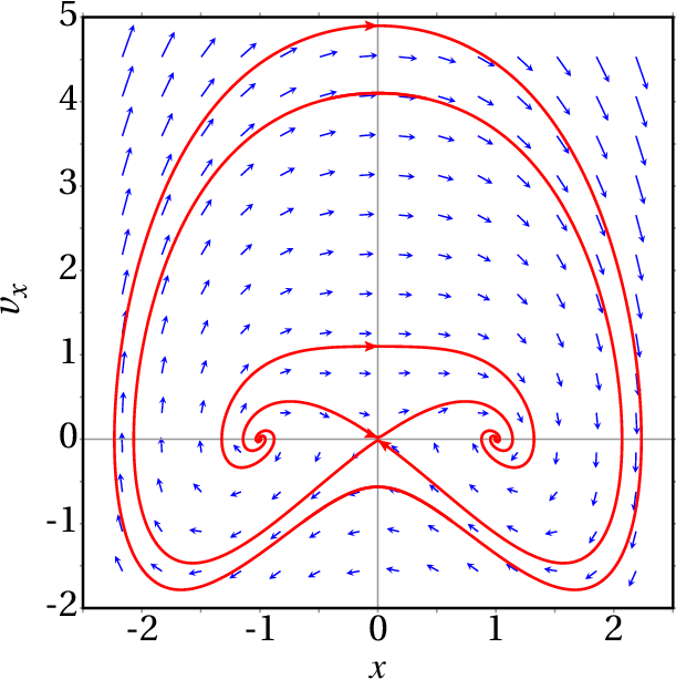
(click to continue)